Download as PDF, PPTX
![ABC model choice via random forests
1 simulation-based methods in
Econometrics
2 Genetics of ABC
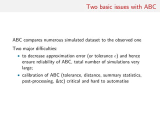
3 Approximate Bayesian computation
4 ABC for model choice
5 ABC model choice via random forests
Random forests
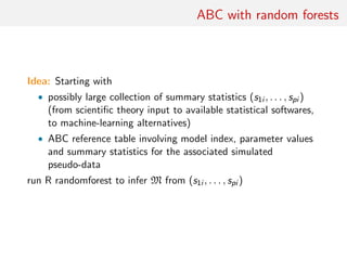
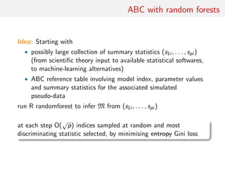
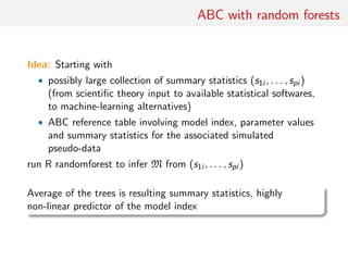
ABC with random forests
Illustrations
6 ABC estimation via random forests
7 [some] asymptotics of ABC](https://image.slidesharecdn.com/abcrafo-170209080838/85/ABC-short-course-final-chapters-1-320.jpg)
![ABC model choice via random forests
1 simulation-based methods in
Econometrics
2 Genetics of ABC
3 Approximate Bayesian computation
4 ABC for model choice
5 ABC model choice via random forests
Random forests
ABC with random forests
Illustrations
6 ABC estimation via random forests
7 [some] asymptotics of ABC](https://image.slidesharecdn.com/abcrafo-170209080838/75/ABC-short-course-final-chapters-1-2048.jpg)
![Leaning towards machine learning
Main notions:
• ABC-MC seen as learning about which model is most
appropriate from a huge (reference) table
• exploiting a large number of summary statistics not an issue
for machine learning methods intended to estimate efficient
combinations
• abandoning (temporarily?) the idea of estimating posterior
probabilities of the models, poorly approximated by machine
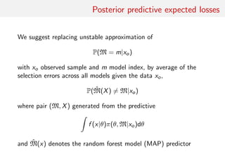
learning methods, and replacing those by posterior predictive
expected loss
[Cornuet et al., 2014, in progress]](https://image.slidesharecdn.com/abcrafo-170209080838/85/ABC-short-course-final-chapters-2-320.jpg)
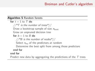
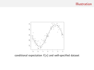
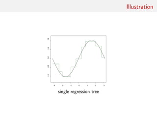
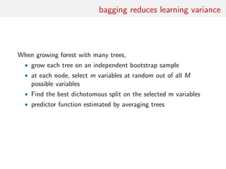
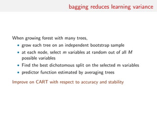
![Random forests
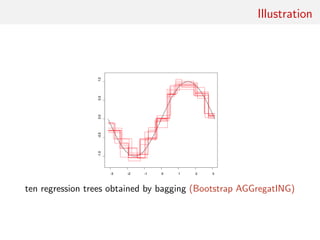
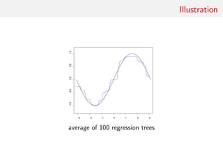
Technique that stemmed from Leo Breiman’s bagging (or
bootstrap aggregating) machine learning algorithm for both
classification and regression
[Breiman, 1996]
Improved classification performances by averaging over
classification schemes of randomly generated training sets, creating
a “forest” of (CART) decision trees, inspired by Amit and Geman
(1997) ensemble learning
[Breiman, 2001]](https://image.slidesharecdn.com/abcrafo-170209080838/85/ABC-short-course-final-chapters-3-320.jpg)
![Growing the forest
Breiman’s solution for inducing random features in the trees of the
forest:
• boostrap resampling of the dataset and
• random subset-ing [of size
√
t] of the covariates driving the
classification at every node of each tree
Covariate xτ that drives the node separation
xτ cτ
and the separation bound cτ chosen by minimising entropy or Gini
index](https://image.slidesharecdn.com/abcrafo-170209080838/85/ABC-short-course-final-chapters-4-320.jpg)
![Subsampling
Due to both large datasets [practical] and theoretical
recommendation from G´erard Biau [private communication], from
independence between trees to convergence issues, boostrap
sample of much smaller size than original data size
N = o(n)](https://image.slidesharecdn.com/abcrafo-170209080838/85/ABC-short-course-final-chapters-6-320.jpg)
![Subsampling
Due to both large datasets [practical] and theoretical
recommendation from G´erard Biau [private communication], from
independence between trees to convergence issues, boostrap
sample of much smaller size than original data size
N = o(n)
Each CART tree stops when number of observations per node is 1:
no culling of the branches](https://image.slidesharecdn.com/abcrafo-170209080838/85/ABC-short-course-final-chapters-7-320.jpg)
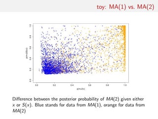
![toy: MA(1) vs. MA(2)
Comparing an MA(1) and an MA(2) models:
xt = t − ϑ1 t−1[−ϑ2 t−2]
Earlier illustration using first two autocorrelations as S(x)
[Marin et al., Stat. & Comp., 2011]
Result #1: values of p(m|x) [obtained by numerical integration]
and p(m|S(x)) [obtained by mixing ABC outcome and density
estimation] highly differ!](https://image.slidesharecdn.com/abcrafo-170209080838/85/ABC-short-course-final-chapters-15-320.jpg)
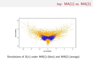
![toy: MA(1) vs. MA(2)
Comparing an MA(1) and an MA(2) models:
xt = t − ϑ1 t−1[−ϑ2 t−2]
Earlier illustration using two autocorrelations as S(x)
[Marin et al., Stat. & Comp., 2011]
Result #2: Embedded models, with simulations from MA(1)
within those from MA(2), hence linear classification poor](https://image.slidesharecdn.com/abcrafo-170209080838/85/ABC-short-course-final-chapters-17-320.jpg)
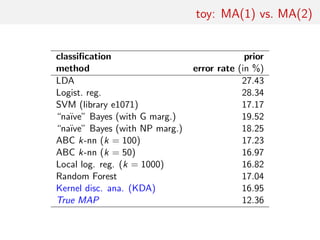
![toy: MA(1) vs. MA(2)
Comparing an MA(1) and an MA(2) models:
xt = t − ϑ1 t−1[−ϑ2 t−2]
Earlier illustration using two autocorrelations as S(x)
[Marin et al., Stat. & Comp., 2011]
Result #3: On such a small dimension problem, random forests
should come second to k-nn ou kernel discriminant analyses](https://image.slidesharecdn.com/abcrafo-170209080838/85/ABC-short-course-final-chapters-19-320.jpg)
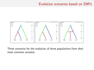
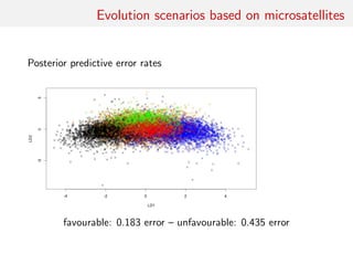
![Evolution scenarios based on SNPs
DIYBAC header (!)
7 parameters and 48 summary statistics
3 scenarios: 7 7 7
scenario 1 [0.33333] (6)
N1 N2 N3
0 sample 1
0 sample 2
0 sample 3
ta merge 1 3
ts merge 1 2
ts varne 1 N4
scenario 2 [0.33333] (6)
N1 N2 N3
..........
ts varne 1 N4
scenario 3 [0.33333] (7)
N1 N2 N3
........
historical parameters priors (7,1)
N1 N UN[100.0,30000.0,0.0,0.0]
N2 N UN[100.0,30000.0,0.0,0.0]
N3 N UN[100.0,30000.0,0.0,0.0]
ta T UN[10.0,30000.0,0.0,0.0]
ts T UN[10.0,30000.0,0.0,0.0]
N4 N UN[100.0,30000.0,0.0,0.0]
r A UN[0.05,0.95,0.0,0.0]
ts>ta
DRAW UNTIL](https://image.slidesharecdn.com/abcrafo-170209080838/85/ABC-short-course-final-chapters-22-320.jpg)
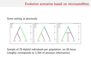
![Evolution scenarios based on SNPs
Model 1 with 6 parameters:
• four effective sample sizes: N1 for population 1, N2 for
population 2, N3 for population 3 and, finally, N4 for the
native population;
• the time of divergence ta between populations 1 and 3;
• the time of divergence ts between populations 1 and 2.
• effective sample sizes with independent uniform priors on
[100, 30000]
• vector of divergence times (ta, ts) with uniform prior on
{(a, s) ∈ [10, 30000] ⊗ [10, 30000]|a < s}](https://image.slidesharecdn.com/abcrafo-170209080838/85/ABC-short-course-final-chapters-23-320.jpg)
![Evolution scenarios based on SNPs
Model 2 with same parameters as model 1 but the divergence time
ta corresponds to a divergence between populations 2 and 3; prior
distributions identical to those of model 1
Model 3 with extra seventh parameter, admixture rate r. For that
scenario, at time ta admixture between populations 1 and 2 from
which population 3 emerges. Prior distribution on r uniform on
[0.05, 0.95]. In that case models 1 and 2 are not embeddeded in
model 3. Prior distributions for other parameters the same as in
model 1](https://image.slidesharecdn.com/abcrafo-170209080838/85/ABC-short-course-final-chapters-24-320.jpg)
![Evolution scenarios based on SNPs
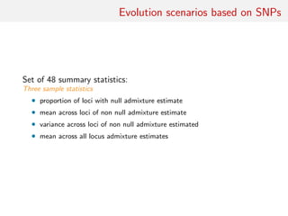
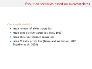
Set of 48 summary statistics:
Single sample statistics
• proportion of loci with null gene diversity (= proportion of monomorphic
loci)
• mean gene diversity across polymorphic loci
[Nei, 1987]
• variance of gene diversity across polymorphic loci
• mean gene diversity across all loci](https://image.slidesharecdn.com/abcrafo-170209080838/85/ABC-short-course-final-chapters-25-320.jpg)
![Evolution scenarios based on SNPs
Set of 48 summary statistics:
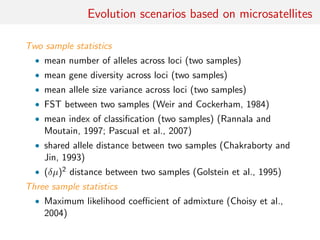
Two sample statistics
• proportion of loci with null FST distance between both samples
[Weir and Cockerham, 1984]
• mean across loci of non null FST distances between both samples
• variance across loci of non null FST distances between both samples
• mean across loci of FST distances between both samples
• proportion of 1 loci with null Nei’s distance between both samples
[Nei, 1972]
• mean across loci of non null Nei’s distances between both samples
• variance across loci of non null Nei’s distances between both samples
• mean across loci of Nei’s distances between the two samples](https://image.slidesharecdn.com/abcrafo-170209080838/85/ABC-short-course-final-chapters-26-320.jpg)
![Evolution scenarios based on SNPs
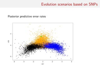
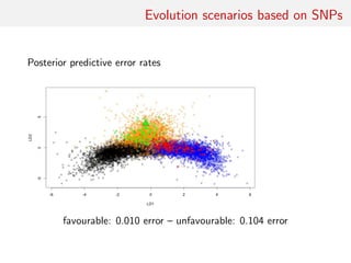
For a sample of 1000 SNIPs measured on 25 biallelic individuals
per population, learning ABC reference table with 20, 000
simulations, prior predictive error rates:
• “na¨ıve Bayes” classifier 33.3%
• raw LDA classifier 23.27%
• ABC k-nn [Euclidean dist. on summaries normalised by MAD]
25.93%
• ABC k-nn [unnormalised Euclidean dist. on LDA components]
22.12%
• local logistic classifier based on LDA components with
• k = 500 neighbours 22.61%
• random forest on summaries 21.03%
(Error rates computed on a prior sample of size 104)](https://image.slidesharecdn.com/abcrafo-170209080838/85/ABC-short-course-final-chapters-28-320.jpg)
![Evolution scenarios based on SNPs
For a sample of 1000 SNIPs measured on 25 biallelic individuals
per population, learning ABC reference table with 20, 000
simulations, prior predictive error rates:
• “na¨ıve Bayes” classifier 33.3%
• raw LDA classifier 23.27%
• ABC k-nn [Euclidean dist. on summaries normalised by MAD]
25.93%
• ABC k-nn [unnormalised Euclidean dist. on LDA components]
22.12%
• local logistic classifier based on LDA components with
• k = 1000 neighbours 22.46%
• random forest on summaries 21.03%
(Error rates computed on a prior sample of size 104)](https://image.slidesharecdn.com/abcrafo-170209080838/85/ABC-short-course-final-chapters-29-320.jpg)
![Evolution scenarios based on SNPs
For a sample of 1000 SNIPs measured on 25 biallelic individuals
per population, learning ABC reference table with 20, 000
simulations, prior predictive error rates:
• “na¨ıve Bayes” classifier 33.3%
• raw LDA classifier 23.27%
• ABC k-nn [Euclidean dist. on summaries normalised by MAD]
25.93%
• ABC k-nn [unnormalised Euclidean dist. on LDA components]
22.12%
• local logistic classifier based on LDA components with
• k = 5000 neighbours 22.43%
• random forest on summaries 21.03%
(Error rates computed on a prior sample of size 104)](https://image.slidesharecdn.com/abcrafo-170209080838/85/ABC-short-course-final-chapters-30-320.jpg)
![Evolution scenarios based on SNPs
For a sample of 1000 SNIPs measured on 25 biallelic individuals
per population, learning ABC reference table with 20, 000
simulations, prior predictive error rates:
• “na¨ıve Bayes” classifier 33.3%
• raw LDA classifier 23.27%
• ABC k-nn [Euclidean dist. on summaries normalised by MAD]
25.93%
• ABC k-nn [unnormalised Euclidean dist. on LDA components]
22.12%
• local logistic classifier based on LDA components with
• k = 5000 neighbours 22.43%
• random forest on LDA components only 23.1%
(Error rates computed on a prior sample of size 104)](https://image.slidesharecdn.com/abcrafo-170209080838/85/ABC-short-course-final-chapters-31-320.jpg)
![Evolution scenarios based on SNPs
For a sample of 1000 SNIPs measured on 25 biallelic individuals
per population, learning ABC reference table with 20, 000
simulations, prior predictive error rates:
• “na¨ıve Bayes” classifier 33.3%
• raw LDA classifier 23.27%
• ABC k-nn [Euclidean dist. on summaries normalised by MAD]
25.93%
• ABC k-nn [unnormalised Euclidean dist. on LDA components]
22.12%
• local logistic classifier based on LDA components with
• k = 5000 neighbours 22.43%
• random forest on summaries and LDA components 19.03%
(Error rates computed on a prior sample of size 104)](https://image.slidesharecdn.com/abcrafo-170209080838/85/ABC-short-course-final-chapters-32-320.jpg)
![Back to Asian Ladybirds [message in a beetle]
Comparing 10 scenarios of Asian beetle invasion beetle moves](https://image.slidesharecdn.com/abcrafo-170209080838/85/ABC-short-course-final-chapters-41-320.jpg)
![Back to Asian Ladybirds [message in a beetle]
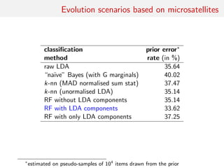
Comparing 10 scenarios of Asian beetle invasion beetle moves
classification prior error†
method rate (in %)
raw LDA 38.94
“na¨ıve” Bayes (with G margins) 54.02
k-nn (MAD normalised sum stat) 58.47
RF without LDA components 38.84
RF with LDA components 35.32
†
estimated on pseudo-samples of 104
items drawn from the prior](https://image.slidesharecdn.com/abcrafo-170209080838/85/ABC-short-course-final-chapters-42-320.jpg)
![Back to Asian Ladybirds [message in a beetle]
Comparing 10 scenarios of Asian beetle invasion beetle moves
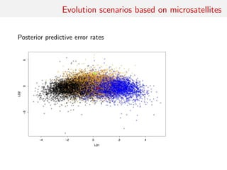
Random forest allocation frequencies
1 2 3 4 5 6 7 8 9 10
0.168 0.1 0.008 0.066 0.296 0.016 0.092 0.04 0.014 0.2
Posterior predictive error based on 20,000 prior simulations and
keeping 500 neighbours (or 100 neighbours and 10 pseudo-datasets
per parameter)
0.3682](https://image.slidesharecdn.com/abcrafo-170209080838/85/ABC-short-course-final-chapters-43-320.jpg)
![Back to Asian Ladybirds [message in a beetle]
Comparing 10 scenarios of Asian beetle invasion](https://image.slidesharecdn.com/abcrafo-170209080838/85/ABC-short-course-final-chapters-44-320.jpg)
![Back to Asian Ladybirds [message in a beetle]
Comparing 10 scenarios of Asian beetle invasion](https://image.slidesharecdn.com/abcrafo-170209080838/85/ABC-short-course-final-chapters-45-320.jpg)
![Back to Asian Ladybirds [message in a beetle]
Comparing 10 scenarios of Asian beetle invasion
0 500 1000 1500 2000
0.400.450.500.550.600.65
k
error
posterior predictive error 0.368](https://image.slidesharecdn.com/abcrafo-170209080838/85/ABC-short-course-final-chapters-46-320.jpg)
![ABC estimation via random forests
1 simulation-based methods in
Econometrics
2 Genetics of ABC
3 Approximate Bayesian computation
4 ABC for model choice
5 ABC model choice via random forests
6 ABC estimation via random forests
7 [some] asymptotics of ABC](https://image.slidesharecdn.com/abcrafo-170209080838/85/ABC-short-course-final-chapters-48-320.jpg)
![classification of summaries by random forests
Given a large collection of summary statistics, rather than selecting
a subset and excluding the others, estimate each parameter of
interest by a machine learning tool like random forests
• RF can handle thousands of predictors
• ignore useless components
• fast estimation method with good local properties
• automatised method with few calibration steps
• substitute to Fearnhead and Prangle (2012) preliminary
estimation of ˆθ(yobs)
• includes a natural (classification) distance measure that avoids
choice of both distance and tolerance
[Marin et al., 2016]](https://image.slidesharecdn.com/abcrafo-170209080838/85/ABC-short-course-final-chapters-50-320.jpg)
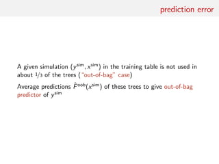
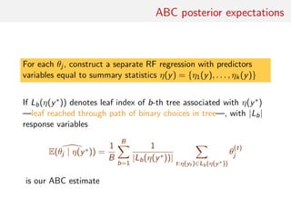
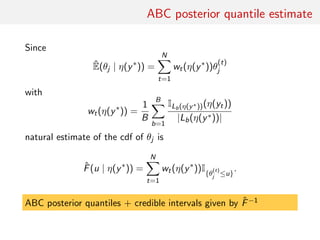
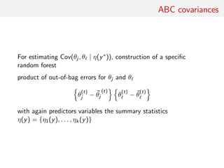
![ABC posterior quantile estimate
Random forests also available for quantile regression
[Meinshausen, 2006, JMLR]
Since
ˆE(θj | η(y∗
)) =
N
t=1
wt(η(y∗
))θ
(t)
j
with
wt(η(y∗
)) =
1
B
B
b=1
ILb(η(y∗))(η(yt))
|Lb(η(y∗))|
natural estimate of the cdf of θj is
ˆF(u | η(y∗
)) =
N
t=1
wt(η(y∗
))I{θ
(t)
j ≤u}
.](https://image.slidesharecdn.com/abcrafo-170209080838/85/ABC-short-course-final-chapters-65-320.jpg)
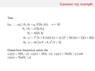
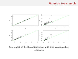
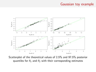
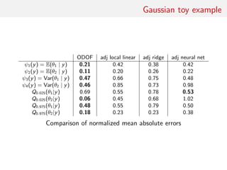
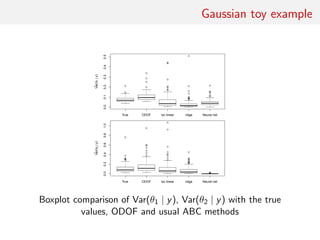
![Gaussian toy example
Reference table of N = 10, 000 Gaussian replicates
Independent Gaussian test set of size Npred = 100
k = 53 summary statistics: the sample mean, the sample
variance and the sample median absolute deviation, and 50
independent pure-noise variables (uniform [0,1])](https://image.slidesharecdn.com/abcrafo-170209080838/85/ABC-short-course-final-chapters-71-320.jpg)
![[some] asymptotics of ABC
1 simulation-based methods in
Econometrics
2 Genetics of ABC
3 Approximate Bayesian computation
4 ABC for model choice
5 ABC model choice via random forests
6 ABC estimation via random forests
7 [some] asymptotics of ABC](https://image.slidesharecdn.com/abcrafo-170209080838/85/ABC-short-course-final-chapters-77-320.jpg)
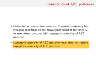
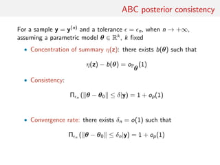
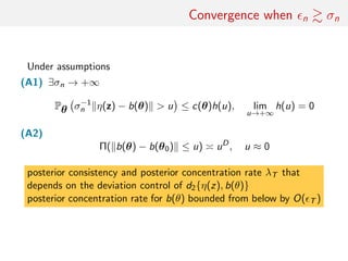
![consistency of ABC posteriors
Asymptotic study of the ABC-posterior z = z(n)
• ABC posterior consistency and convergence rate (in n)
• Asymptotic shape of π (·|y(n))
• Asymptotic behaviour of ˆθ = EABC[θ|y(n)]
[Frazier et al., 2016]](https://image.slidesharecdn.com/abcrafo-170209080838/85/ABC-short-course-final-chapters-78-320.jpg)
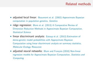
![Related results
existing studies on the large sample properties of ABC, in which
the asymptotic properties of point estimators derived from ABC
have been the primary focus
[Creel et al., 2015; Jasra, 2015; Li & Fearnhead, 2015]](https://image.slidesharecdn.com/abcrafo-170209080838/85/ABC-short-course-final-chapters-81-320.jpg)
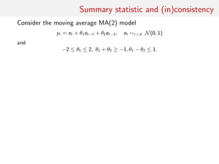
![Summary statistic and (in)consistency
Consider the moving average MA(2) model
yt = et + θ1et−1 + θ2et−2, et ∼i.i.d. N(0, 1)
and
−2 ≤ θ1 ≤ 2, θ1 + θ2 ≥ −1, θ1 − θ2 ≤ 1.
summary statistics equal to sample autocovariances
ηj (y) = T−1
T
t=1+j
yt yt−j j = 0, 1
with
η0(y)
P
→ E[y2
t ] = 1 + (θ01)2
+ (θ02)2
and η1(y)
P
→ E[yt yt−1] = θ01(1 + θ02)
For ABC target pε (θ|η(y)) to be degenerate at θ0
0 = b(θ0) − b (θ) =
1 + (θ01)2
+ (θ02)2
θ01(1 + θ02)
−
1 + (θ1)2
+ (θ2)2
θ1(1 + θ2)
must have unique solution θ = θ0
Take θ01 = .6, θ02 = .2: equation has 2 solutions
θ1 = .6, θ2 = .2 and θ1 ≈ .5453, θ2 ≈ .3204](https://image.slidesharecdn.com/abcrafo-170209080838/85/ABC-short-course-final-chapters-90-320.jpg)

![main result
Set Σn(θ) = σnD(θ) for θ ≈ θ0 and Zo = Σn(θ0)−1(η(y) − θ0),
then under (B1) and (B2)
• when nσ−1
n → +∞
Π n [ −1
n (θ − θ0) ∈ A|y] ⇒ UB0 (A), B0 = {x ∈ Rk
; b (θ0)T
x ≤ 1}
• when nσ−1
n → c
Π n [Σn(θ0)−1
(θ − θ0) − Zo
∈ A|y] ⇒ Qc(A), Qc = N
• when nσ−1
n → 0 and (B3) holds, set
Vn = [b (θ0)]T
Σn(θ0)b (θ0)
then
Π n [V −1
n (θ − θ0) − ˜Zo
∈ A|y] ⇒ Φ(A),](https://image.slidesharecdn.com/abcrafo-170209080838/85/ABC-short-course-final-chapters-93-320.jpg)
![intuition
Set x(θ) = σ−1
n (θ − θ0) − Zo (k = 1)
πn := Π n [ −1
n (θ − θ0) ∈ A|y]
=
|θ−θ0|≤un
1lx(θ)∈A
Pθ σ−1
n (η(z) − b(θ)) + x(θ) ≤ σ−1
n n p(θ)dθ
|θ−θ0|≤un
Pθ σ−1
n (η(z) − b(θ)) + x(θ) ≤ σ−1
n n p(θ)dθ
+ op(1)
• If n/σn 1 :
Pθ |σ−1
n (η(z) − b(θ)) + x(θ)| ≤ σ−1
n n = 1+o(1), iff |x| ≤ σ−1
n
• If n/σn = o(1)
Pθ |σ−1
n (η(z) − b(θ)) + x| ≤ σ−1
n n = φ(x)σn(1 + o(1))](https://image.slidesharecdn.com/abcrafo-170209080838/85/ABC-short-course-final-chapters-94-320.jpg)
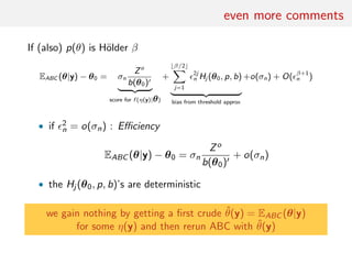
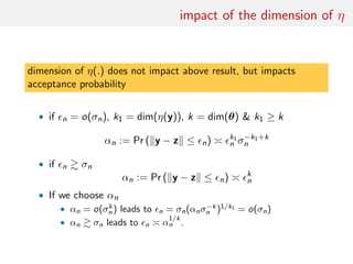
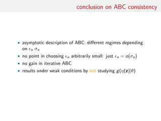
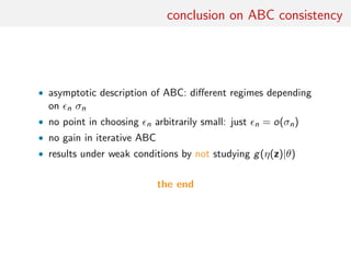

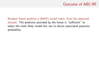
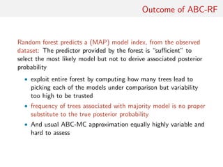
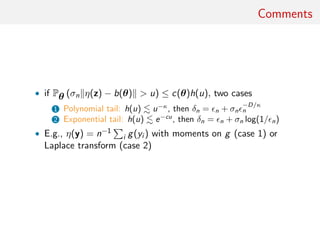
The document discusses using random forests for approximate Bayesian computation (ABC) model choice. It proposes: 1. Using random forests to infer a model from summary statistics, as random forests can handle a large number of statistics and find efficient combinations. 2. Replacing estimates of posterior model probabilities, which are poorly approximated, with posterior predictive expected losses to evaluate models. 3. An example comparing MA(1) and MA(2) time series models using two autocorrelations as summaries, finding embedded models and that random forests perform similarly to other methods on small problems.


![Inference in generative models using the Wasserstein distance [[INI]](https://cdn.slidesharecdn.com/ss_thumbnails/inewton-170706120746-thumbnail.jpg?width=640&height=640&fit=bounds)


