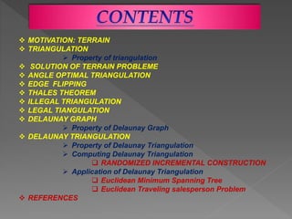
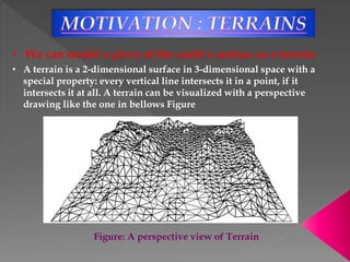
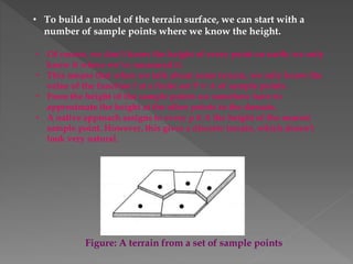
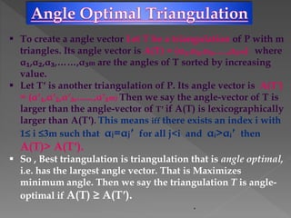
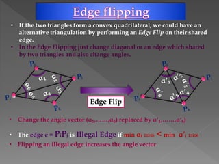
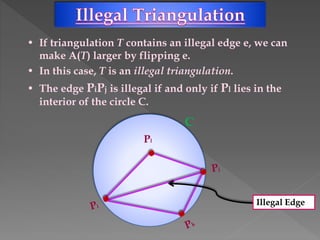
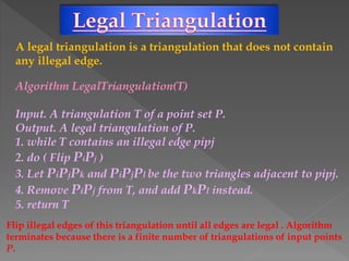
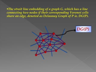
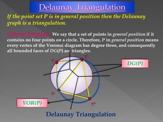
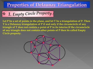
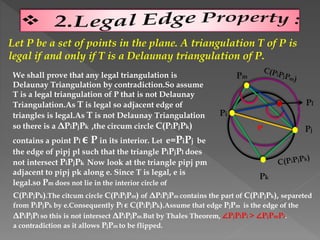
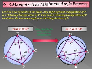
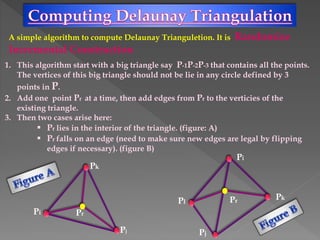
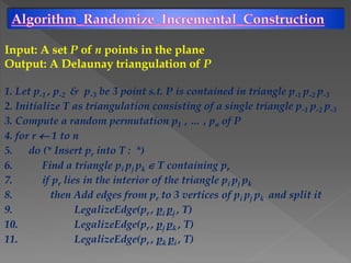
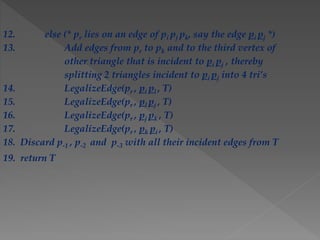
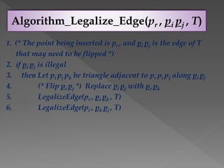
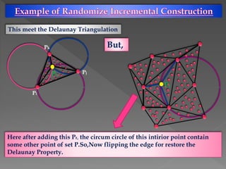
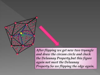
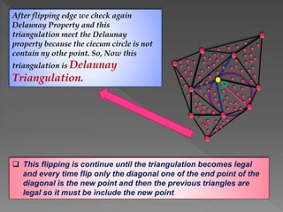
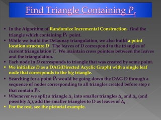
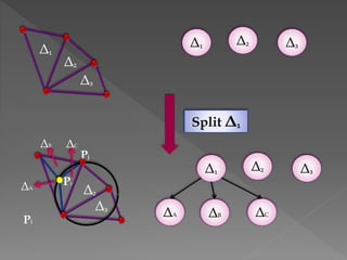
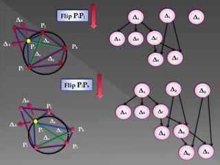
The document discusses Delaunay triangulation, which is a method for generating a triangulation of a set of points in a plane. It begins by motivating the problem of modeling a terrain from sample height points. It then discusses using triangulations to approximate the terrain, and defines properties of triangulations. It introduces the concept of Delaunay triangulation, which maximizes the minimum angle of all possible triangulations. It describes an algorithm called randomized incremental construction that computes the Delaunay triangulation by incrementally adding points and maintaining the Delaunay property through edge flips.

1. Boris N.Delaunay

2.  MOTIVATION: TERRAIN
 TRIANGULATION
 Property of triangulation
 SOLUTION OF TERRAIN PROBLEME
 ANGLE OPTIMAL TRIANGULATION
 EDGE FLIPPING
 THALES THEOREM
 ILLEGAL TRIANGULATION
 LEGAL TIANGULATION
 DELAUNAY GRAPH
 Property of Delaunay Graph
 DELAUNAY TRIANGULATION
 Property of Delaunay Triangulation
 Computing Delaunay Triangulation
 RANDOMIZED INCREMENTAL CONSTRUCTION
 Application of Delaunay Triangulation
 Euclidean Minimum Spanning Tree
 Euclidean Traveling salesperson Problem
 REFERENCES

3. • We can model a piece of the earth’s surface as a terrain.
• A terrain is a 2-dimensional surface in 3-dimensional space with a
special property: every vertical line intersects it in a point, if it
intersects it at all. A terrain can be visualized with a perspective
drawing like the one in bellows Figure
Figure: A perspective view of Terrain

4. • To build a model of the terrain surface, we can start with a
number of sample points where we know the height.
• Of course, we don’t know the height of every point on earth; we only
know it where we’ve measured it.
• This means that when we talk about some terrain, we only know the
value of the function f at a finite set P ⊂ A of sample points.
• From the height of the sample points we somehow have to
approximate the height at the other points in the domain.
• A native approach assigns to every p ∈ A the height of the nearest
sample point. However, this gives a discrete terrain, which doesn’t
look very natural.
Figure: A terrain from a set of sample points

5. So, How can we most naturally approximate height
of points not in A?
• Determine a
Triangulation of A in
R², then raise points to
desired height
• Triangulation: planar
subdivision whose
bounded faces are
triangles with vertices
from A
Figure : Triangulation

6. Maximal planar subdivision: a subdivision S such that
no edge connecting two vertices can be added to S without
destroying its planarity
Triangulation of set of points P: a maximal planar
subdivision whose vertices are elements of P.
Plane Graph: No two edges in the embedding cross.

7. • Outer polygon must be
convex hull that is the
union of the bounded faces
of T is always the convex
hull of P, and that the
unbounded face is always
the complement of the
convex hull.
• Internal faces must be
triangles, otherwise they
could be triangulated
further. Convex Hull

8. Here, Some triangles are better than other in triangulation.
SO, now remain a question that-
But which triangulation is the most appropriate one for
our purpose, namely to approximate a terrain??
• There is no definitive answer to this question. We do not know the
original terrain, we only know its height at the sample points.
Since we have no other information, and the height at the sample
points is the correct height for any triangulation, all triangulations
of P seem equally good. Nevertheless, some triangulations look
more natural than others.
• So here we will avoid skinny triangles. That means we will try
maximize the minimum angles which is basically DELAUNAY
TRIANGULATION
SO, TERRAIN Problem solve by Angle Optimal
Triangulation(Edge Flipping) and Delaunay Triangulation

9.  To create a angle vector Let T be a triangulation of P with m
triangles. Its angle vector is A(T) = (α₁,α₂,α₃,.....,α₃m) where
α₁,α₂,α₃,……,α₃m are the angles of T sorted by increasing
value.
 Let Tʹ is another triangulation of P. Its angle vector is A(Tʹ)
= (αʹ₁,αʹ₂,αʹ₃,.......,αʹ₃m) Then we say the angle-vector of T is
larger than the angle-vector of Tʹ if A(T) is lexicographically
larger than A(Tʹ). This means iff there exists an index i with
1≤ i ≤3m such that αj=αjʹ for all j<i and αᵢ>αᵢʹ then
A(T)> A(Tʹ).
 So , Best triangulation is triangulation that is angle optimal,
i.e. has the largest angle vector. That is Maximizes
minimum angle. Then we say the triangulation T is angle-
optimal if A(T) ≥ A(Tʹ).
.

10. • If the two triangles form a convex quadrilateral, we could have an
alternative triangulation by performing an Edge Flip on their shared
edge.
• In the Edge Flipping just change diagonal or an edge which shared
by two triangles and also change angles.
Edge Flip
• Change the angle vector (α₁,……,α₆) replaced by αʹ₁,……,αʹ₆)
• The edge e = PiPj is Illegal Edge if min αᵢ 1≤i≤6 < min α’ᵢ 1≤i≤6
• Flipping an illegal edge increases the angle vector

11. • We can use Thale’s Theorem to test if an edge is legal
without calculating angles
Denote the smaller angle
defined by three points p, q,
r.
Let C be a circle, l a line
intersecting C in points a and
b and p, q, r, and s points
lying on the same side of l.
Suppose that p and q lie on C,
that r lies inside C, and that s
lies outside C. Then:

12. • If triangulation T contains an illegal edge e, we can
make A(T) larger by flipping e.
• In this case, T is an illegal triangulation.
• The edge PiPj is illegal if and only if Pl lies in the
interior of the circle C.
Pl
Illegal Edge
C

13. A legal triangulation is a triangulation that does not contain
any illegal edge.
Algorithm LegalTriangulation(T)
Input. A triangulation T of a point set P.
Output. A legal triangulation of P.
1. while T contains an illegal edge pipj
2. do ( Flip PiPj )
3. Let PiPjPk and PiPjPl be the two triangles adjacent to pipj.
4. Remove PiPj from T, and add PkPl instead.
5. return T
Flip illegal edges of this triangulation until all edges are legal . Algorithm
terminates because there is a finite number of triangulations of input points
P.

14. The strait line embedding of a graph G, which has a line
connecting two nodes if their corresponding Voronoi cells
share an edge, denoted as Delaunay Graph of P ie. DG(P).
DG(P)

15. • No two edges cross; DG(P) is a planar graph.
 PiPj is in DG(P) iff ∃ closed disc Cij
with Pi and Pjon the boundary and no
other site is contained in it.
 Let tij be the triangle formed by Pi,Pj
and center of Cij.
 Note that edge of tij between Pi and
center of Cij is inside V(Pi).
 Let another edge PkPl also in DG(P)
such that PiPj and PkPl
intersect.Define Ckl and tkl for PkPl.If
intersected PiPj, it must also intersect
one other edge e of tij.Because Pk Contained in v(Pi)
Contained in v(Pi)
 and Pl are outside Cij and therefore outside tij.Say an edge e’ of tkl must
intersect PiPj.
 Notice that one of the edges of tij incident to center of Cij and one of the edges
of tkl incident to center of Ckl must intersect.
 But, those edges must be contained within their respective Voronoi cells,
which is a contradiction.

16. If the point set P is in general position then the Delaunay
graph is a triangulation.
General Position: We say that a set of points in general position if it
contains no four points on a circle. Therefore, P in general position means
every vertex of the Voronoi diagram has degree three, and consequently
all bounded faces of DG(P) are triangles.
Delaunay Triangulation
DG(P)
VOR(P)

17. Let P be a set of points in the plane, and let T be a triangulation of P. Then
T is a Delaunay triangulation of P if and only if the circumcircle of any
triangle of T does not contain a point of P in its interior.If the circumcircle
of any triangle does not contain other points of P then its called Empty
Circle property.

18. Let P be a set of points in the plane. A triangulation T of P is
legal if and only if T is a Delaunay triangulation of P.
We shall prove that any legal triangulation is
Delaunay Triangulation by contradiction.So assume
T is a legal triangulation of P that is not Delaunay
Triangulation.As T is legal so adjacent edge of
triangles is legal.As T is not Delaunay Triangulation
so there is a ΔPiPjPk ,the circum circle C(PiPjPk)
contains a point Pl ϵ P in its interior. Let e=PiPj be
the edge of pipj pl such that the triangle PiPjPl does
not intersect PiPjPk Now look at the triangle pipj pm
adjacent to pipj pk along e. Since T is legal, e is
legal.so Pm does not lie in the interior circle of
Pm
Pk
Pj
Pi
Pl
C(PiPjPk).The citcum circle C(PiPjPm) of ΔPiPjPm contains the part of C(PiPjPk), separeted
from PiPjPk by e.Consequently Pl ϵ C(PiPjPk).Assume that edge PjPm is the edge of the
ΔPiPjPl so this is not intersect ΔPiPjPm.But by Thales Theorem, ∠PjPlPi > ∠PjPmPi.
a contradiction as it allows PjPm to be flipped.

19. Let P be a set of points in the plane. Any angle-optimal triangulation of P
is a Delaunay Triangulation of P. That is any Delaunay triangulation of P
maximizes the minimum angle over all triangulations of P.
A
B
C
D
90°
A
B
C
D
min αᵢ = 27° min αᵢ = 50°After edge flip for
angle optimal
triangulation

20. • If we can verify for every edges that the two triangles are sharing the
edges are legal then it if Delaunay Triangulation.
• We can’t take every circum circle and check the respectively point.
But we only look at the edge which is sharing the two triangles and
draw the circum circles if they are not contain any other point and
this is holds for every pair of trianngles then it’s a Delaunay
Triangulation. This is called Local Property

21. 1. This algorithm start with a big triangle say P-1P-2P-3 that contains all the points.
The vertices of this big triangle should not be lie in any circle defined by 3
points in P.
2. Add one point Pr at a time, then add edges from Pr to the verticies of the
existing triangle.
3. Then two cases arise here:
 Pr lies in the interior of the triangle. (figure: A)
 Pr falls on an edge (need to make sure new edges are legal by flipping
edges if necessary). (figure B)
Pi
Pj
Pk
Pr
Pk
Pj
Pl
Pi
Pr
A simple algorithm to compute Delaunay Trianguletion. It is Randomize
Incremental Construction

22. Input: A set P of n points in the plane
Output: A Delaunay triangulation of P
1. Let p-1 , p-2 & p-3 be 3 point s.t. P is contained in triangle p-1 p-2 p-3
2. Initialize T as triangulation consisting of a single triangle p-1 p-2 p-3
3. Compute a random permutation p1 , … , pn of P
4. for r  1 to n
5. do (* Insert pr into T : *)
6. Find a triangle pi pj pk  T containing pr
7. if pr lies in the interior of the triangle pi pj pk
8. then Add edges from pr to 3 vertices of pi pj pk and split it
9. LegalizeEdge(pr , pi pj , T)
10. LegalizeEdge(pr , pj pk , T)
11. LegalizeEdge(pr , pk pi , T)

23. 12. else (* pr lies on an edge of pi pj pk, say the edge pi pj *)
13. Add edges from pr to pk and to the third vertex of
other triangle that is incident to pi pj , thereby
splitting 2 triangles incident to pi pj into 4 tri’s
14. LegalizeEdge(pr , pi pl , T)
15. LegalizeEdge(pr , pl pj , T)
16. LegalizeEdge(pr , pj pk , T)
17. LegalizeEdge(pr , pk pi , T)
18. Discard p-1 , p-2 and p-3 with all their incident edges from T
19. return T

24. Algorithm_Legalize_Edge(pr , pi pj , T)
1. (* The point being inserted is pr , and pi pj is the edge of T
that may need to be flipped *)
2. if pi pj is illegal
3. then Let pi pj pk be triangle adjacent to pr pi pj along pi pj
4. (* Flip pi pj *) Replace pi pj with pr pk
5. LegalizeEdge(pr , pi pk , T)
6. LegalizeEdge(pr , pk pj , T)

25. Pi
Pr
Pk
Pj
This meet the Delaunay Triangulation
Here after adding this Pr, the circum circle of this intirior point contain
some other point of set P.So,Now flipping the edge for restore the
Delaunay Property.
But,
Pr

26. After flipping we get new two tryangle
and draw the circum circle and check
the Delaunay Property,but this figure
again not meet the Delaunay
Property.So we flipping the edge again.
P
r

27. After flipping edge we check again
Delaunay Property and this
triangulation meet the Delaunay
property because the ciecum circle is not
contain ny othe point. So, Now this
triangulation is Delaunay
Triangulation.
 This flipping is continue until the triangulation becomes legal
and every time flip only the diagonal one of the end point of the
diagonal is the new point and then the previous triangles are
legal so it must be include the new point
P
r

28.  In the Algorithm of Randomize Incremental Construction , find the
triangle which containing Pr point.
 While we build the Delaunay triangulation, we also build a point
location structure D. The leaves of D correspond to the triangles of
current triangulation T. We maintain cross pointers between the leaves
and the triangulation.
 Each node in D corresponds to triangle that was created by some point.
 We initialize D as a DAG(Directed Acyclic Graph) with a single leaf
node that corresponds to the big triangle.
 Searching for a point Pr would be going down the DAG D through a
sequence of nodes corresponding to all triangles created before step r
that contain Pr.
 Whenever we split a triangle 1 into smaller triangles a and b (and
possibly c), add the smaller triangles to D as leaves of 1
 For the rest, see the pictorial example.

29. Δ₁
Δ₂
Δ₃
Δ₂ Δ₃Δ₁
ΔA
Δ₂
Δ₃
Δ₂ Δ₃Δ₁
ΔB ΔC
Pr
ΔCΔBΔA
Pj
Pi
Split Δ₁

30. Δ₄
Δ₅
Δ₃
Δ₂ Δ₃Δ₁
ΔCΔBΔA
ΔA
ΔB
Pr
Δ5
Δ4
Pj
Pi
Pk
Δ₄
Δ₆
Δ₇
Δ₂ Δ₃Δ₁
ΔCΔBΔA
ΔA
ΔB
Pr Δ₅Δ₄
Pj
Pi
Pk
Δ₇Δ₆
Pl
Flip PiPj
Flip PiPk

31. Let M be the maximum value of any
coordinate of a point in P. Then , big
the triangle has the vertices at
P-1 = (3M, 0),
P-2 = (0, 3M)
and
P-3 = (- 3M, - 3M).
This are not actual coordinate.
M
M

32. The Randomized Incremental Algorithm for the Delaunay
Triangulation of n points takes O(n log n) time and O(n)
space, both on expectation.
From nodes in D representing triangles created .Each triangle takes O(1) time, so
the total time will be O(n) + (time for point locations).
Now Searching for a point Pr would entail going down the DAG D through a
sequence of nodes corresponding to all triangles created before step r that
contain Pr.
So each triangle that was created is visited once for each point in it. In other
words, . . . Let K(∆) ⊆ P be the points inside triangle ∆. Time for point locations is
∆
K(∆)
each triangle created in round r has O(n/r) points of P in it. Therefore,
∆
K(∆) ≤
𝒓
O(n/r)
ϵ O n(log n)

33.  Euclidean Minimum Spanning Trees
For a set P of n points in the plane, the
Euclidean Minimum Spanning Tree is the
graph with minimum summed edge length
that connects all points in P and has only
the points of P as vertices
 The Euclidean Minimum
Spanning Tree does not have
cycles.
 Suppose G is the shortest connected
graph and it has a cycle. Removing one
edge from the cycle makes a new graph
G0 that is still connected but which is
shorter. Contradiction
Euclidean Minimum
Spanning Tree

34.  Every edge of the Euclidean Minimum Spanning Tree is an
edge in the Delaunay graph
• Suppose T is an EMST with an
edge e = pq that is not Delaunay
Consider the circle C that has e as
its diameter. Since e is not
Delaunay, C must contain another
point r in P.
• Either the path in T from r to p
passes through q, or vice versa.
The cases are symmetric, so we
can assume the former case.
• Then removing e and inserting pr
instead will give a connected
graph again (in fact, a tree)
• Since q was the furthest point
from p inside C, r is closer to q, so
T was not a minimum spanning
tree. Contradiction
P
q
r
e
T
Which is not
possible
T’

35. A data structure exists that maintains disjoint sets and allows the following two
operations:
Union: Takes two sets and makes one new set that is the union.
Find: Takes one element and returns the name of the set that contains it
If there are n elements in total, then all Unions together take O(nlogn) time and each
Find operation takes O(1) time
Let P be a set of n points in the plane for which we want to compute the
EMST
1. Make a Union-Find structure where every point of P is in a separate set
2. Construct the Delaunay triangulation DT of P
3. Take all edges of DT and sort them by length
4. For all edges e from short to long:
Let the endpoints of e be p and q
If Find(p) ≠ Find(q), then put e in the EMST, and
Union(Find(p),Find(q))
So, The Euclidean Minimum Spanning Tree of P can be computed in O(nlogn)
time

36. • Given a set P of n points in the plane, the Euclidean Traveling
Salesperson Problem is to compute a tour (cycle) that visits all points of P
and has minimum length . A tour is an order on the points of P (cyclic
order). A set of n points has (n-1)! different tours
• We can determine the length of each tour in O(n) time: a brute-force
algorithm to solve the Euclidean Traveling Salesperson Problem (ETSP)
takes O(n) O((n-1)!) = O(n!) time
• If an algorithm A solves an optimization problem always within a factor
k of the optimum, then A is called an k-approximation algorithm.
• If an instance I of ETSP has an optimal solution of length L, then a k-
approximation algorithm will and a tour of length ≤ k L

37. We will use the EMST to approximate the ETSP
start at any vertexfollow an edge on one sideto get to another vertexproceed this wayskipping visited verticesand close the tour

38. • The walk visits every edge twice,
so it has length 2│EMST│
• The tour skips vertices, which
means the tour has length ≤
2│EMST│
• The optimal ETSP-tour is a
spanning tree if you remove any
edge!!!
So │EMST│ < │ETSP│
• Remove the edge PiPj . So now this
ETSP is EMST.
Pi
Pj
 A tour visiting all points whose length is at most twice the
minimum possible can be computed in O(nlogn) time. So an
O(nlogn) time, 2-approximation for ETSP exists
 As ETMST is meet the Delaunay property and evry edges are Delaunay
edges then ETSP is also meet Delaunay Property and its edges are
Delaunay edges

39. DOCUMENTS:
 E:PGSEM 3SEMINERDelaunay2D.ppt
 E:PGSEM 3SEMINERComputing the Delunay Triangulation.ppt
 E:PGSEM 3SEMINERinterpolation.pdf
 E:PGSEM 3SEMINERDELAUNAY TRIANGULATION.mp4
WEBSITES
 https://en.wikipedia.org/wiki/Delaunay_triangulation
 http://www.cs.uu.nl/docs/vakken/ga/slides9alt.pdf
 http://www.cse.iitm.ac.in/~augustine/cs6100_even2012/slides/09_Delau
nayTriangulation.pdf
 https://www.youtube.com/watch?v=IqdSdbxrTsY