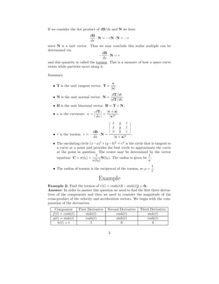
- The binormal vector B(t) is defined as the cross product of the unit tangent vector T(t) and unit normal vector N(t).
- It is proven that B(t) is a unit vector, meaning it has constant length. Its derivative dB/ds is therefore orthogonal to B(t).
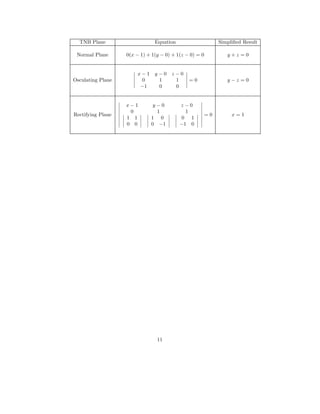
- The torsion τ of a space curve is defined as the rate of change of the binormal vector with respect to arc length s, or τ = -dB/ds·N. Torsion measures how much a curve twists as one moves along it.
- For a plane curve, the torsion is always zero since the cross product that defines torsion is equal to the
![Unit Binormal Vector B and Torsion
If r(t) is a smooth space curve, |T(t)| = 1 for all t, we have T′
and T are
orthogonal.
Proof: Since the tangent vector, T, is of constant length (recall that |T(t)| = 1
so it is of constant length) we have
T · T = c2
d
dt
[T · T] = 0
T′
· T + T · T′
= 0
2T′
· T = 0
and since the dot product between two vectors is zero implies the vectors are
orthogonal, we have our result.
Note that T′
(t) is not necessarily a unit vector, but if r′
(t) is also smooth
then the unit tangent and unit normal vectors can be defined as:
T =
v
|v|
N =
T′
|T′
|
.
The last vector in the TNB frame is called the binormal vector. It is perpendic-
ular to both the T(t) and N(t) vectors and is also a unit vector. It is computed
via the cross product of the unit tangent and the unit normal vectors. Thus:
B(t) = T(t) × N(t)
Below we prove the binormal vector is a unit vector.
Proof that B is a unit vector: We have
|B(t)| = |T(t) × N(t)|
= |T||N| sin(θ)
= (1)(1) sin(π/2)
= 1
Thus, the binormal vector is also a unit vector. This also establishes that the
binormal has constant length. Hence its derivative will also be orthogonal to it.
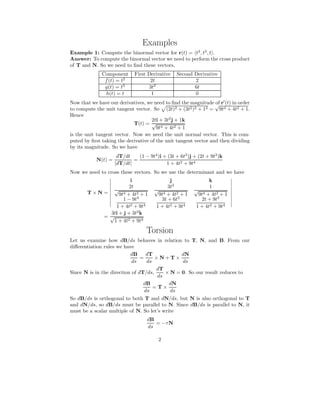
Because we are evaluating several cross products and we typically use deter-
minants to do these evaluations, let us review how to interpret the determinant
notation for 2 × 2 and 3 × 3 matrices:
a b
c d
= ad − bc
a b c
d e f
g h i
= aei + bfg + cdh − ceg − fha − idb
1](https://image.slidesharecdn.com/61cc98ed-d2f0-4da8-8f4a-7361f2180fe0-150412130104-conversion-gate01/85/torsionbinormalnotes-1-320.jpg)
![Unit Binormal Vector B and Torsion
If r(t) is a smooth space curve, |T(t)| = 1 for all t, we have T′
and T are
orthogonal.
Proof: Since the tangent vector, T, is of constant length (recall that |T(t)| = 1
so it is of constant length) we have
T · T = c2
d
dt
[T · T] = 0
T′
· T + T · T′
= 0
2T′
· T = 0
and since the dot product between two vectors is zero implies the vectors are
orthogonal, we have our result.
Note that T′
(t) is not necessarily a unit vector, but if r′
(t) is also smooth
then the unit tangent and unit normal vectors can be defined as:
T =
v
|v|
N =
T′
|T′
|
.
The last vector in the TNB frame is called the binormal vector. It is perpendic-
ular to both the T(t) and N(t) vectors and is also a unit vector. It is computed
via the cross product of the unit tangent and the unit normal vectors. Thus:
B(t) = T(t) × N(t)
Below we prove the binormal vector is a unit vector.
Proof that B is a unit vector: We have
|B(t)| = |T(t) × N(t)|
= |T||N| sin(θ)
= (1)(1) sin(π/2)
= 1
Thus, the binormal vector is also a unit vector. This also establishes that the
binormal has constant length. Hence its derivative will also be orthogonal to it.
Because we are evaluating several cross products and we typically use deter-
minants to do these evaluations, let us review how to interpret the determinant
notation for 2 × 2 and 3 × 3 matrices:
a b
c d
= ad − bc
a b c
d e f
g h i
= aei + bfg + cdh − ceg − fha − idb
1](https://image.slidesharecdn.com/61cc98ed-d2f0-4da8-8f4a-7361f2180fe0-150412130104-conversion-gate01/75/torsionbinormalnotes-1-2048.jpg)