The definite integral is defined as the limit of Riemann sums as the norm of the partition approaches 0. A Riemann sum is the sum of the areas of rectangles formed by the function over subintervals of its domain. The definite integral calculates the signed area between the function's graph and the x-axis over an interval. It generalizes the idea of finding the area under a curve to allow for functions that are negative, discontinuous, or unbounded over the interval.

1. 8|The Definite Integral
Chapter 2
The Definite Integral
2.1 Introduction to Area
Two problems, both from geometry, motivate the two most important ideas in
calculus. The problem of finding the tangent line led us to the derivative. The
problem of finding area will lead us to the definite integral. For polygons (closed
plane regions hounded by line segments), the problem of finding area is hardly a
problem at all. We start by defining the area of a rectangle to be the familiar length
times width, and from this we successively derive the formulas for the area of a
parallelogram, a triangle, and any polygon. The sequence of figures in Figure 1
suggests how this is done. Even in this simple setting, it is clear that area should
satisfy five properties.
1. The area of a plane region is a nonnegative (real) number.
2. The area of a rectangle is the product of its length and width (both measured
in the same units). The result is in square units, for example, square feet or
square centimeters.
3.
Congruent regions have equal areas.
4. The area of the union of two regions that overlap only in a line segment is the
sum of the areas of the two regions.
5.
If one region is contained in a second region, then the area of the first region
is less than or equal to that of the second.
Figure 1

2. 9|The Definite Integral
When we consider a region with a curved boundary, the problem of assigning
area is more difficult. However, over 2000 years ago Archimedes provided the key
to a solution. Consider a sequence of inscribed polygons that approximate the curved
region with greater and greater accuracy. For example, for the circle of radius 1,
consider regular inscribed polygons
with 4 sides, 8 sides, 16 sides, ... , as
shown in Figure 2. The area of the circle is the limit as
of the areas of
.
Thus, if A(F) denotes the area of a region F. Then
(circle)
Figure 2
Archimedes went further, considering also circumscribed polygons
(Figure 3). He showed that you get the same value for the area of the circle of radius
1 (what we call ) whether you use inscribed or circumscribed polygons. It is just a
small step from what he did to our modern treatment of area.
Figure 3

3. 10 | T h e D e f i n i t e I n t e g r a l
Sigma Notation
Our approach to finding the area of a curved region R will involve the
following steps:
1. Approximate the region R by n rectangles where the n rectangles taken together
either contain R. producing a circumscribed polygon, or are contained in R,
producing an inscribed polygon.
2. Find the area of each rectangle.
3. Sum the areas of the n rectangles.
4. Take the limit as
If the limit of areas of inscribed and circumscribed polygons is the same, we call this
limit the area of the region R. Step 3, involving summing the areas of rectangles,
requires us to have a notation for summation, as well as some of its properties.
Consider, for example, the following sums:
and
To indicate these sums in a compact way. We write these sums as
respectively. Here
(capital Greek sigma), which corresponds to the English S,
says that we are to sum (add) all numbers of the form indicated as the
runs
through the positive integers, starting with the integer shown below and ending with
the integer above
If all the
in
. Thus,
have the same value, say c, then

4. 11 | T h e D e f i n i t e I n t e g r a l
As a result,
In particular,
Properties of
Thought of as an operator,
operates on sequences, and it does so in a linear way
Teorema 2.1: Linearity of ∑
Proof
The proofs are easy; we consider only (i)
EXAMPLE 2.1
SOLUTION

5. 12 | T h e D e f i n i t e I n t e g r a l
EXAMPLE 2.2
Show that :
SOLUTION
a. Here we should resist our inclination to apply linearity and instead write out the
sum, hoping for some nice cancellations
b. This follows immediately from part (a).
The symbol used for the index does not matter. Thus,
and all of these are equal to
. For this reason, the index is
sometimes called a dummy index.
Some Special Sum Formulas
When finding areas of regions we will often need to consider the sum of the
first a positive integers, as well as the sums of their squares, cubes, and so on. There
are nice formulas for these; proofs are discussed after Example 2.4.

6. 13 | T h e D e f i n i t e I n t e g r a l
EXAMPLE 2.3
Find a formula for
SOLUTION We make use of linearity and Formulas 1 and 2 from above.
EXAMPLE 2.4
How many oranges are in the pyramid shown in Figure 4?
Figure 4
SOLUTION

7. 14 | T h e D e f i n i t e I n t e g r a l
Proofs of Special Sum Formulas
To prove Special Sum
—
Formula 1, we
start
with
the identity
, sum both sides, apply Example 2 on the left, and use
linearity on the right.
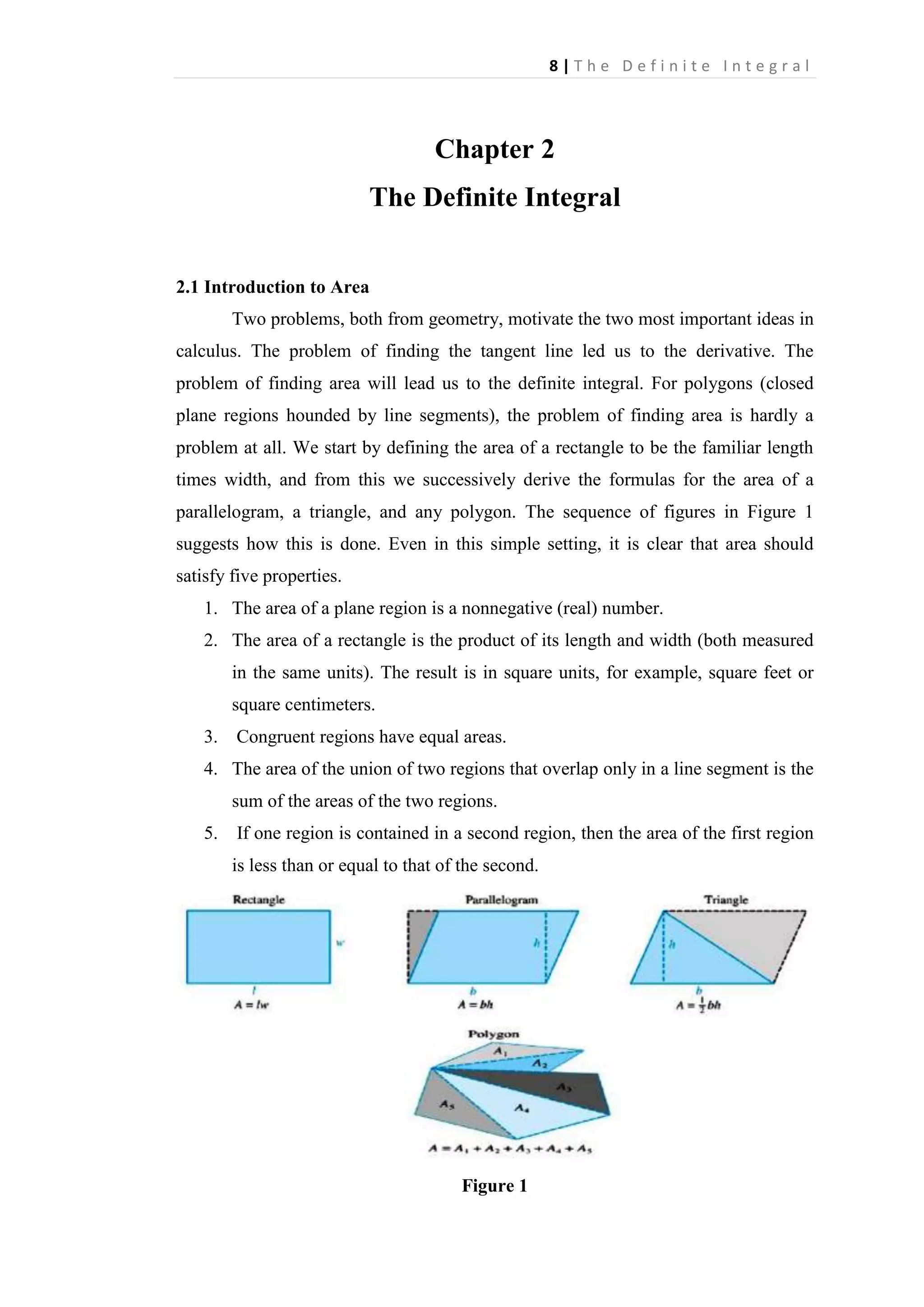
Area by Inscribed Polygons
Consider the region R bounded by the parabola
-axis, and the vertical line
curve
between
, the
(Figure 5). We refer to R as the region under the
and
Figure 5
. Our aim is to calculate its area
Figure 6
Partition (as in Figure 6) the interval [0, 2] into n subintervals, each of length
by means of the
Thus
points

8. 15 | T h e D e f i n i t e I n t e g r a l
Consider the typical angle with base
is f
and height
. Its area
(see the upper-left part of Figure 7), The union k of all such rectangles
forms the inscribed polygon shown in the lower-right part of Figure 7, The area
A(
) can be calculated by summing the areas of these rectangles.
Now
Thus,
We conclude that

9. 16 | T h e D e f i n i t e I n t e g r a l
Figure 7
The diagrams in Figure 8 should help you to visualize what is happening as a gets
larger and larger.
Figure 8

10. 17 | T h e D e f i n i t e I n t e g r a l
Area by Circumscribed Polygons
Perhaps you are still not convinced that
. We can give more evidence.
Consider the rectangle with base
and height
(shown at the
upper left in Figure 9). Its area is
. The union S, of all such rectangles
forms a circumscribed polygon for the region R, as shown at the lower right in
Figure 9.
Figure 9
The area
is calculated in analogy with the calculation of A
As before,
and so
Again, we conclude that

11. 18 | T h e D e f i n i t e I n t e g r a l
Exercises 2.1
In Problems 1-5, find the value of the indicated sum
1.
2.
3.
4.
5.
In Problems 6-9, write the indicated sum in sigma notation
6.
7.
8.
9.
In Problems 10-13, suppose that
Calculate each of the following
10.
11.
In Problem 12-15, use Special Sum Formula 1-4 to find each
12.
13.
14.
15.

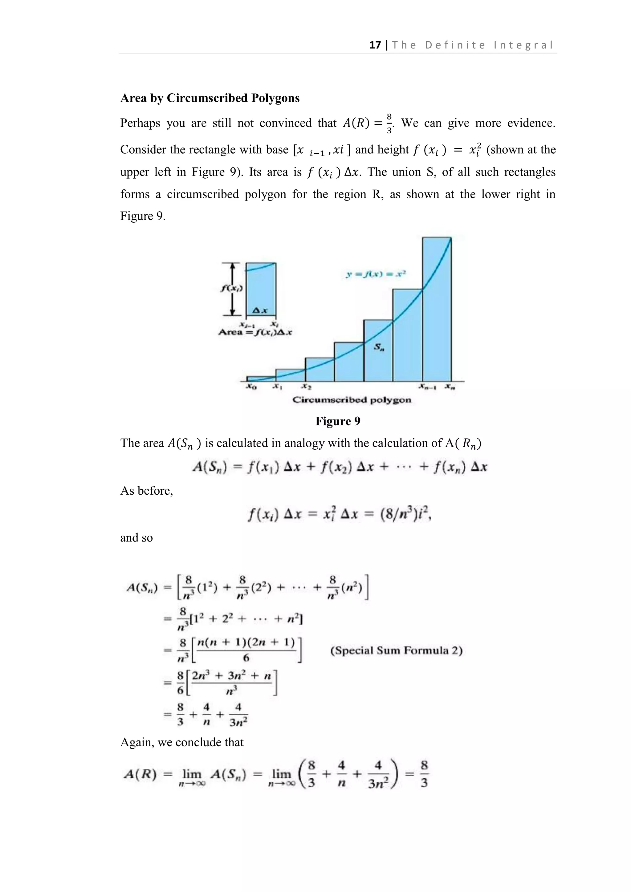
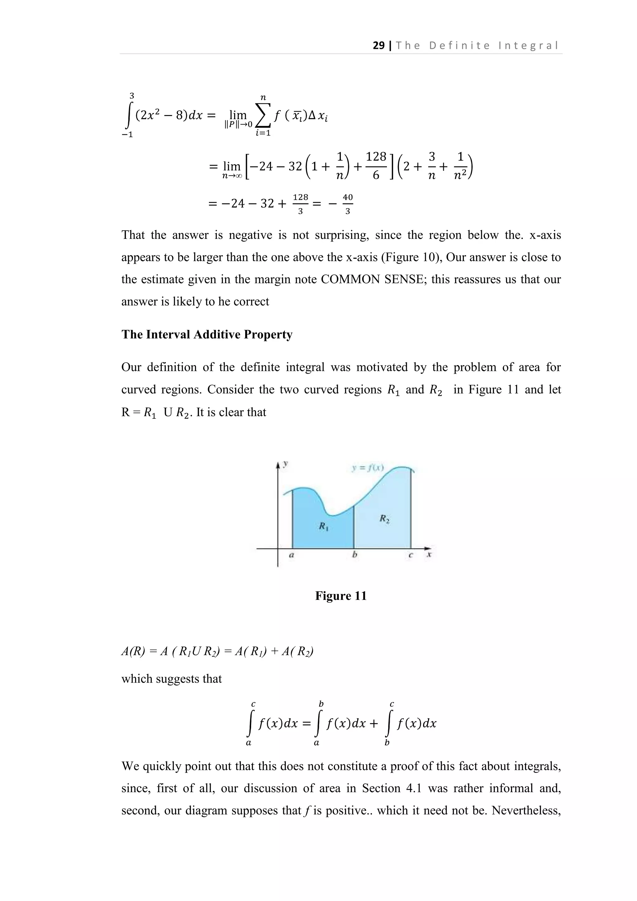
12. 19 | T h e D e f i n i t e I n t e g r a l
2.2 The Definite Integral
All the preparations have been made; we are ready to define the definite integral. The
Definite Integral Both Newton and Leibniz introduced early versions of this concept.
However, it was Georg Friedrich Bernhard Riernann (1826-1866) who gave us the
modern definition. In formulating this definition, we are guided by the ideas we
discussed in the previous section. The first notion is that of a Riemann sum.
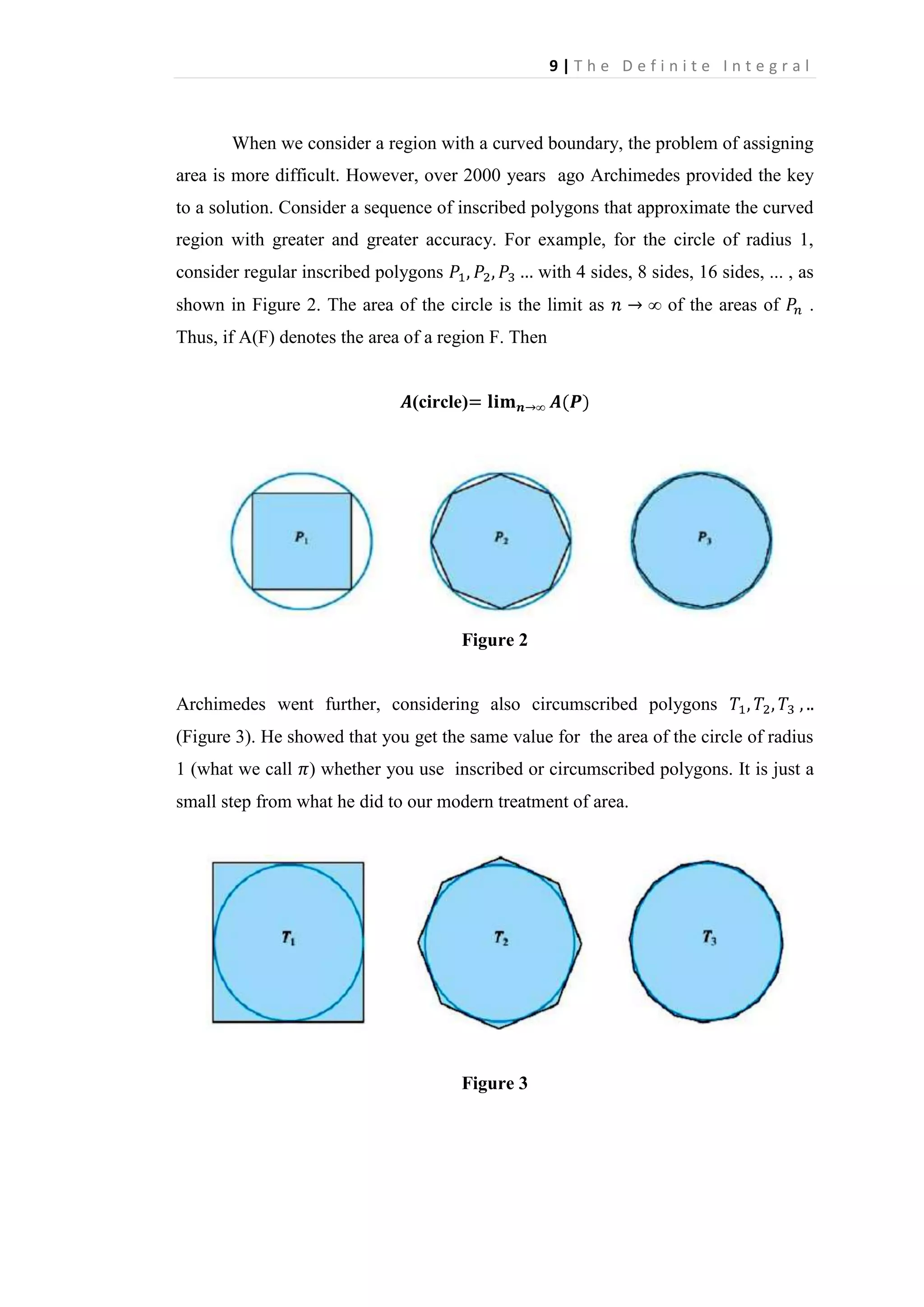
Rieffiami Sums
Consider a function f defined on a closed interval [a, b]. It may have both positive
and negative values on the interval, and it does not even need to be continuous. Its
graph might look something like the one in Figure 1.
Figure 1
Consider a partition P of the interval [a, h] into n subintervals (not necessarily
of equal length) by means of points
and let
On each subinterval [
], pick an arbitrary point
(which may be an end point); we call it a sample point for the ith subinterval. An
example of these constructions is shown in Figure 2 for n = 6.
A Partition of [a,b] with Sample points
Figure 2

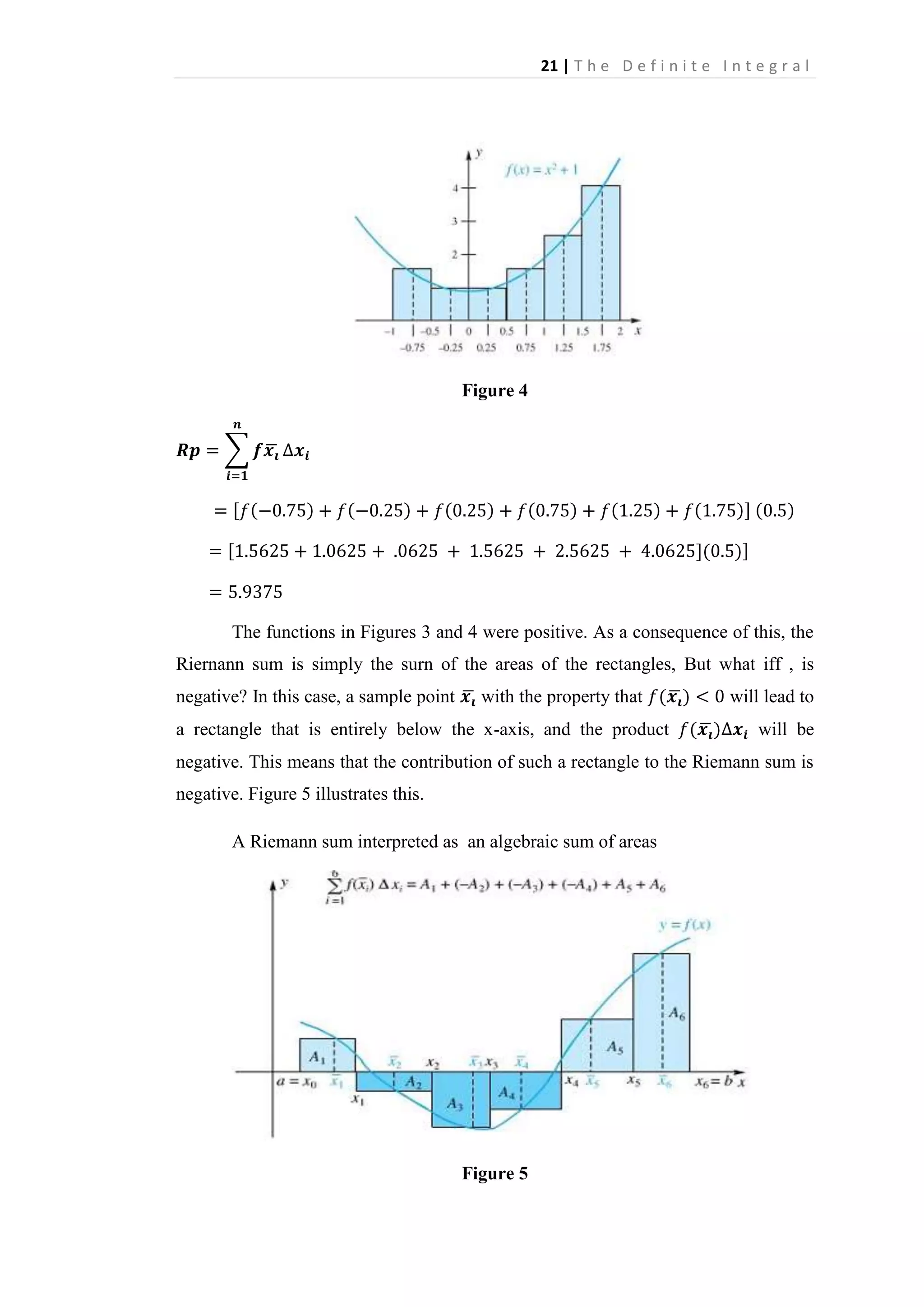
13. 20 | T h e D e f i n i t e I n t e g r a l
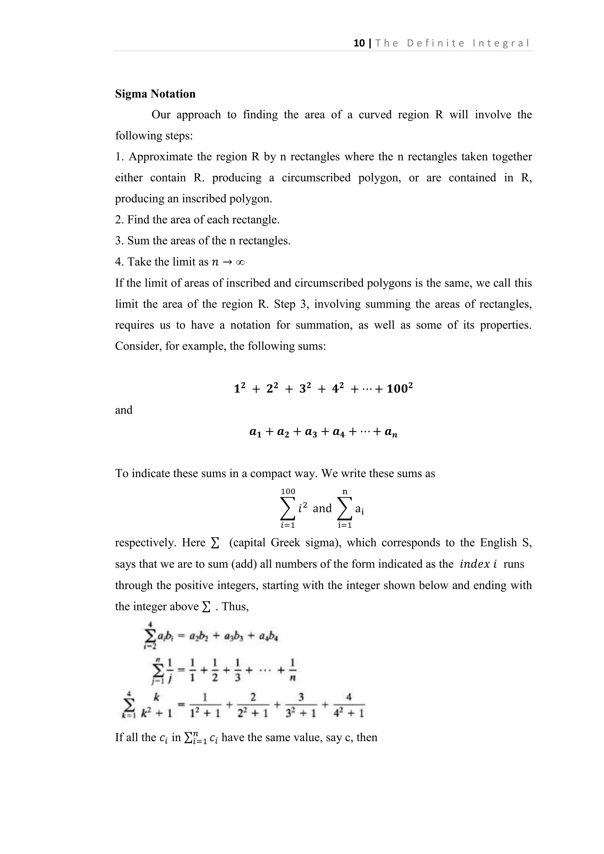
We call the sum
a Riemann sum for f corresponding to the partition P. Its geometric interpretation
is shown in Figure 3.
A Riemann sum interpreted as an algebraic sum of areas
y
Figure 3
EXAMPLE 3.1
Evaluate the Riemann sum for
on the interval [-1, 2] using the
equally spaced partition points -1 < -0.5 < 0 < 0.5 < 1 < 1.5 < 2, with the sample
point
being the midpoint of the ith subinterval.
SOLUTION
Note the picture in Figure 4.

14. 21 | T h e D e f i n i t e I n t e g r a l
Figure 4
The functions in Figures 3 and 4 were positive. As a consequence of this, the
Riernann sum is simply the surn of the areas of the rectangles, But what iff , is
negative? In this case, a sample point
with the property that
a rectangle that is entirely below the x-axis, and the product
will lead to
will be
negative. This means that the contribution of such a rectangle to the Riemann sum is
negative. Figure 5 illustrates this.
A Riemann sum interpreted as an algebraic sum of areas
Figure 5

15. 22 | T h e D e f i n i t e I n t e g r a l
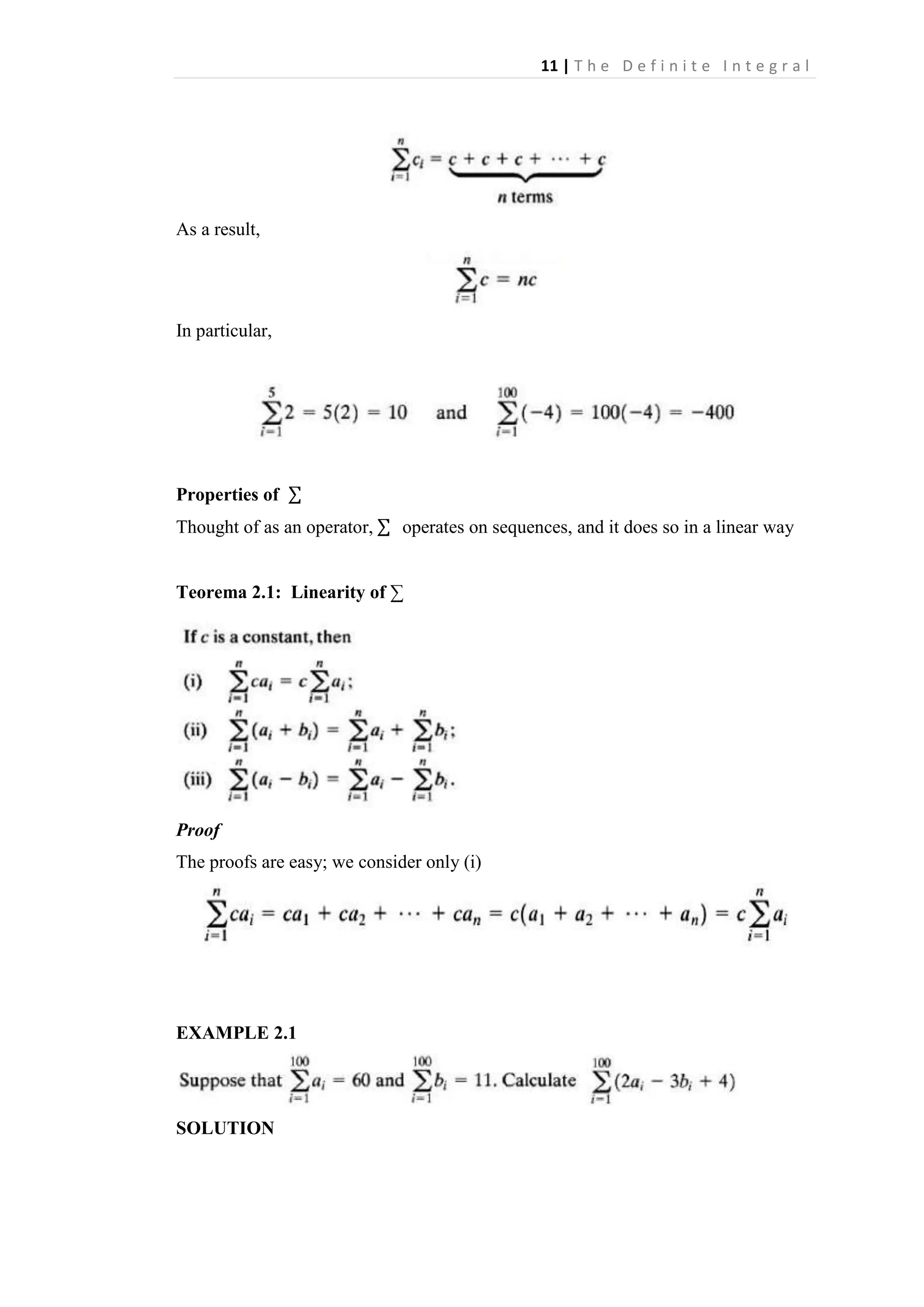
EXAMPLE 2.2 Evaluate the Riemann sum Rp for
on the interval [0, 5] using the partition P with partition points 0 < 1.1 < 2 < 3.2 < 4 <
5 and the corresponding sample points
= 1.5,
= 2.5,
=3.6,
SOLUTION
—
—
= (7.875)(1.1) + (3.125)(O.9) + (-2.625)(1.2) + (-2.944)(0.8) + 18(1)
= 23.9698
The corresponding geometric picture appears in Figure 6.
Figure 6
Definition of the Definite Integral
Suppose now that
and
have the meanings discussed above. Also let
,
called the norm of P, denote the length of the longest of the subintervals of the
partition P. For instance, in Example 1,
= 0,5; in Example 2
= 3,2 - 2 = 1,2.

16. 23 | T h e D e f i n i t e I n t e g r a l
Definition 3.1 Definite Integral
Let f be a function that is defined on the closed interval [a,b]. If
exists, we say f that is iniegrable on [a,b]. Moreover,
, called the definite
integral (or Riemann integral) of f from a to b, is then given by
The heart of the definition is the final line. The concept. captured in that
equation grows out of our discussion of area in the previous section. However, we.
Have considerably modified the notion presented there. For example, we now allow
f to be negative on part or all of [a,b], we use partitions with subintervals that may he
of unequal length, and we allow to be any point on the ith subinterval. Since we have
made these changes, it is important to state precisely how the definite integral relates
to area. In general,
gives the signed area of the region trapped between
the curve y = f(x) and the x-axis on the interval [a, b], meaning that a positive sign is
attached to areas of parts above the x-axis, and a negative sign is attached to areas of
parts below the x-axis. In symbols,
where
and
are as shown in Figure 7.
Figure 7
The meaning of the word limit in the definition of the definite integral is
more general than in earlier usage and should be explained. The equality

17. 24 | T h e D e f i n i t e I n t e g r a l
means that corresponding, to each
for all Riernann sums
for
, there is a
> 0 such that
on [a, b] for which the norm
= of the
associated partition is less than 6. In this case, we say that the indicated limit exists
and has the value L.
That was a mouthful, and we are not going to digest it just now. We simply
assert that the usual limit theorems also hold for this kind of limit.
Returning to the symbol
, we might call a the lower end point and
b' the upper end point for the integral. However, most authors use the terminology
lower limit of integration and upper limit of integration, which is tine provided we
realize that this usage of the word limit has nothing to do with its more technical
meaning.
In our definition of
, we implicitly assumed that a < b. We
remove that restriction with the following definitions.
Thus.
Finally, we point out that x is a dummy variable in the symbol
.
By this lyre mean that x can be replaced by any other letter (provided, of course, that
it is replaced in each place where. it occurs). Thus,

18. 25 | T h e D e f i n i t e I n t e g r a l
What Functions Are Integrable? Not every function is integrable on a closed
interval [a1 b]. For example., the unbounded function
which is graphed in Figure 8, is not integrable on [-2, 2], It can be shown that for
this unbounded function, the Riemann sum can be made arbitrarily large. Therefore,
the limit of the Riemann sum over [-2, 2] does not exist.
Figure 8
Even some bounded functions can fail to be integrable, but they have to be pretty
complicated (see Problem 39 for one example). Theorem 3.1 (below) is the most
important theorem about integrability. Unfortunately.. it is too difficult to prove here:
we leave that for advanced calculus books.
Theorem 3.1 Integrability Theorem
If f is bounded on[a,b] and if it is continuous there except at a finite number of
points, then f is integrable on [a,b]. In particular, if f is continuous on the whole
interval [a,b], it is integrable on [a,b].

19. 26 | T h e D e f i n i t e I n t e g r a l
As a consequence of this theorem, the following functions are integrable on
every closed interval [a, b].
1. Polynomial functions
2. Sine and cosine functions
3. Rational functions, provided that the interval [a, b ] contains no points where the.
denominator is 0.
Calculating Definite Integrals
Knowing that a function is integrable allows us to calcalte its integral by using a
regular partition (i.e., a partition with equal-length subintervals) and by picking the
sample points 1 in any way that is convenient for us. Examples 3 and 4 involve
polynomials, which we just learned are integrable.
EXAMPLE 3 Evaluate
SOLUTION Partition the interval [-2,3] into n equal subintervals, each of length
In each subinterval [xi _ j, xj. use ,Ti = xi as the sample point.
Then
Thus,

20. 27 | T h e D e f i n i t e I n t e g r a l
Since P is a regular partition,
is equivalent to
We conclude that
We can easily check our answer, since the required integral gives the area of
the trapezoid in Figure 9, The familiar trapezoidal area formula
gives
.
Figure 9

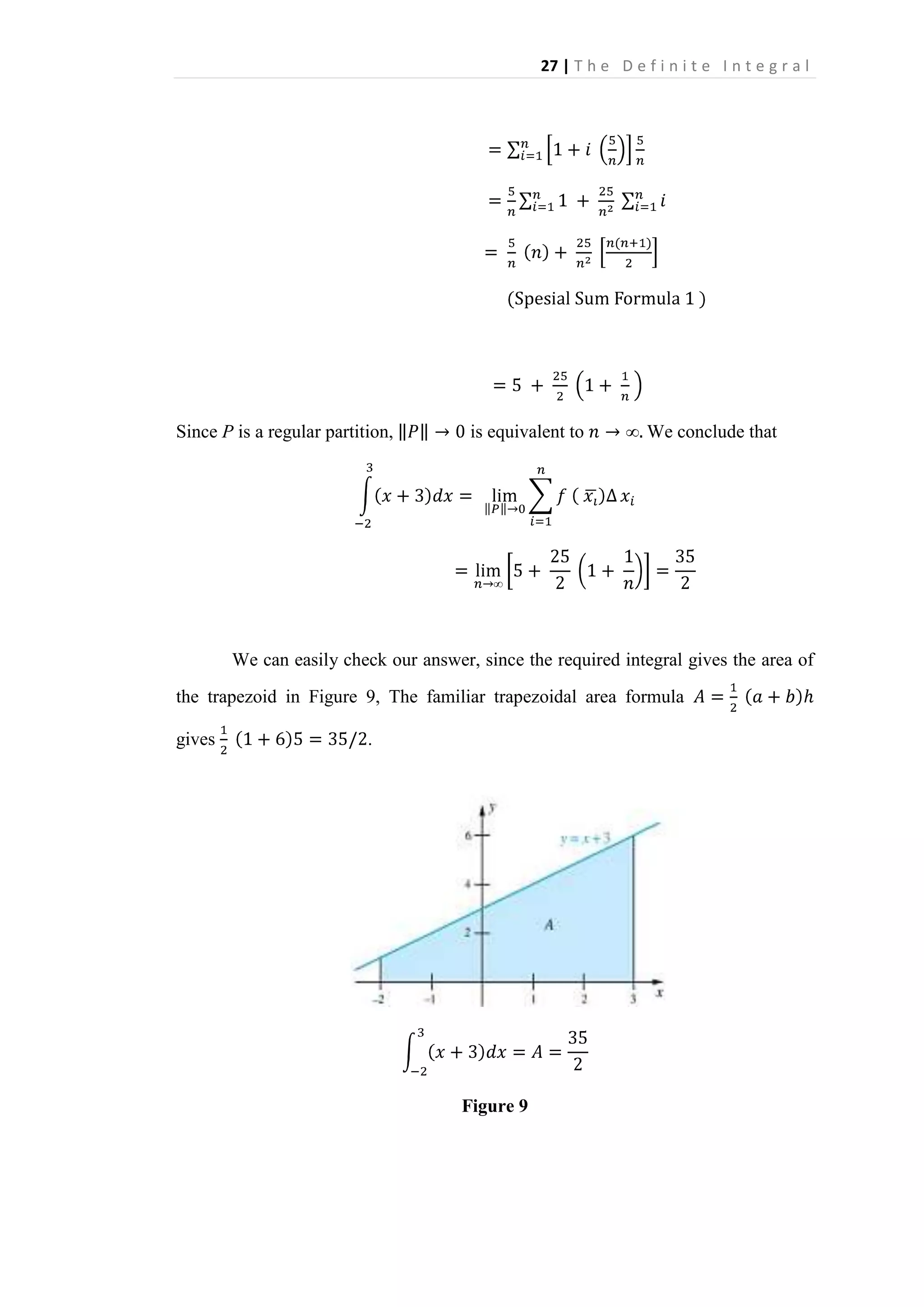
21. 28 | T h e D e f i n i t e I n t e g r a l
EXAMPLE 4 Evaluate
SOLUTION No formulas from elementary geometry will help here. Figure 10
suggests that the integral is equal to
, where
and
are the areas of the
regions below and above the x-axis.
Figure 10
Let P be a regular partition of [-1, 3] into n equal subintervals, each of length
In each subinterval
],choose
. Then
and
Consequently,
=
We conclude that
to be the. right end point, so

22. 29 | T h e D e f i n i t e I n t e g r a l
That the answer is negative is not surprising, since the region below the. x-axis
appears to be larger than the one above the x-axis (Figure 10), Our answer is close to
the estimate given in the margin note COMMON SENSE; this reassures us that our
answer is likely to he correct
The Interval Additive Property
Our definition of the definite integral was motivated by the problem of area for
curved regions. Consider the two curved regions
R=
U
and
in Figure 11 and let
. It is clear that
Figure 11
A(R) = A ( R1U R2) = A( R1) + A( R2)
which suggests that
We quickly point out that this does not constitute a proof of this fact about integrals,
since, first of all, our discussion of area in Section 4.1 was rather informal and,
second, our diagram supposes that f is positive.. which it need not be. Nevertheless,

23. 30 | T h e D e f i n i t e I n t e g r a l
definite in do satisfy this in additive property, and they do it no matter how the three
points a, b, and c are arranged. We leave the rigorous proof to more advanced works.
Theorem 3.2 Interval Additive property
If f is integrable on an interval containing the points a, b, and c, then
no matter what the order of a, b, and c.
For example,
which most people readily believe. But it is also true that
which may seem surprising. If you mistrust the theorem, you might actually evaluate
each of the above integrals to see that the equality holds.
Velocity and Position
Near the end of Section 4.1 we explained how the area under the velocity curve is
equal to the distance traveled, provided the velocity function v(t) is positive. In
general, the position (which could be positive , or negative) is equal to the definite
integral of the velocity function (which could he positive or negative). More
specifically, if v(t) is the velocity of an object at time t, where t
0, and. if the object
is at position 0 at time 0, then the position of the object at time a is
EXAMPLE 5 An object at the origin at time t = 0 has velocity, measured in meters
per second.

24. 31 | T h e D e f i n i t e I n t e g r a l
Sketch the velocity curve. Express the object's position at t = 140 as a definite
integral and evaluate it using formulas from plane geometry.
SOLUTION
Figure 12 shows the velocity curve. The position at time 140 is equal to the definite
integral
which we can evaluate using formulas for the area of a triangle
and a rectangle and using the Interval Additive Property (Theorem 3.2):
Figure 12

25. 32 | T h e D e f i n i t e I n t e g r a l
Exercises 2.2
In Problems 1 and 2, calculate the Riemann sum suggested by each figure
In Problem 3-6, calculate the Riemann sum
3.
4.
.
In Problems 5-7, use the given values of a and b and express the given limit as a
definite integral.
5.
6.
7.
Evaluate the definite integral using the definition, as in Examples 3.3 and 3.4.
8.
9.
10.

26. 33 | T h e D e f i n i t e I n t e g r a l
2.3 The First Fundamental Theorem of Calculus
Calculus is the study of limits, and the two most important limits that you have
studied so far are the derivative and the definite integral. The derivative of a function
f is
and the definite integral is
These two kinds of limits appear to have no connection whatsoever. There is,
however, a very close. connection, as we shall see in this section.
Newton and Leibniz are usually credited with the. simultaneous but
independent discovery of calculus. Yet, the concepts of the slope of a tangent line
(which led to the derivative) were known earlier, having been studied by Blaise
Pascal and Isaac Barrow years before Newton and Leibniz, And Archimedes had
studied areas of curved regions 1800 years earlier, in the third century B.C. by then
do Newton and Leibniz get the credit? They understood kind exploited the intimate
relationship between antiderivatiTves and definite integrals. This important
relationship is called the First Fundamental Theorem of Calculus.
The First Fundamental Theorem
You have likely net several “fundo-m e n tal theorems" in your mathematical career.
The Fundamental Theorem of Arithmetic says that a whole number factors uniquely
into a product of primes. The Fundamental 'Theorem of Algebra says that an nthegree polynomial has n roots, counting complex roots and multiplicities. Any
"fundamental theorem" should be studied carefully, and then permanently committed
to memory.
Near the end of Section 4.1, we studied a problem in which the velocity of an
object at time t is given by
from time t = 0 to time t = 3 is equal to
We found that the distance traveled

27. 34 | T h e D e f i n i t e I n t e g r a l
Using the terminology from Section 4.2, we now see that the distance traveled from
time t = 0 to time t = 3 is equal to the definite integral
(Since the velocity is positive for all
, the distance traveled through time t is
equal to the position of the object at time t, If the velocity were negative for some
value of t, then the object would be traveling backward at that time t; in such a case,
distance traveled would not equal position.) We could use the same. Reasoning to
find that the distance s traveled from time t = 0 to time t = x is
The question we now pose is this: What is the derivative of s?
Since the derivative of distance traveled (as long as the velocity is always
positive) is the velocity, we have
In other words,
Now, define A(x) to be the area under the graph of
i-axis, and between the vertical lines t = 1 and t= x, where
y + above the
(see Figure 1). A
function such as this is called an accumulation function because it accumulates area
under a curve from a fixed value (t = 1 in this case) to a variable value (t = x in this
case). What is the derivative of A?
The area A(x) is equal to the definite integral

28. 35 | T h e D e f i n i t e I n t e g r a l
In this case we can evaluate this definite integral using a geometrical argument; A(x)
is just the area of a trapezoid, so
With this done, we see that the derivative of A is
In other words,
Let's define another accumulation function B as the area under the curve
, above the t-axis, to the right of the origin, and to the left of the line
.
Figure 2
where
see Figure 2). This area is given by the definite integral
. To
find this area, we first construct a Rie.mann sum. We use a regular partition of [0,x]
and evaluate the. function at the right end point of each subinterval. Then
the right end point of the ith interval is
therefore
and
= ix/n. The Riemann sum is

29. 36 | T h e D e f i n i t e I n t e g r a l
The definite integral is the limit of these Riemann sums.
Thus, B(x) =
In other words,
The results of the last three boxed equations suggest that the derivative of an
accumulation function is equal to the function being accumulated. But is this always
the. case? And by should this be the case?
Suppose that we are using a -retractable" paintbrush to paint the region under
a curve, (By retractable, we mean that the brush becomes wider or narrower as it
moves left to right so that it just covers the height to be painted. The brush is wide
when the integrancl values are large and narrow when the integrand values are small.
See Figure 3.) With this analogy, the accumulated area is the painted area, and the
rate of accumulation is the rate at which the. paint is being applied. But the rate at

30. 37 | T h e D e f i n i t e I n t e g r a l
which paint is being applied is equal to the width of the brush.. in effect, the height
of the function. We can restate this result as follows,
The rate of accumulation at t = x is equal to the value of the function being
accumulated at t = x.
Figure 3
This, in a nu[shell, is the First Fundamental Theorem of Calculus it is fUndamental
because it links the derivative and the definite integral, the most important kinds
of limits you have studied so far.
Theorem 3.3 First Fundamental Theorem of Calculus
Let f be continuous on the closed interval [a,b] and let x be a (variable) point in
(a,b). Then
Sketch or Proof For now. we present a sketch of the proof. This sketch shows the
important features of the proof, but a complete proof must wait until after we have
established a few other results. For x in [a, b], define
. Then for x
in (a ,b)

31. 38 | T h e D e f i n i t e I n t e g r a l
The last line follows from the Interval Additive Property (Theorem 4.2B). Now,
when h is small., f does not change. much over the interval [x, x + h]. On this
interval, f is roughly equal to ,f( x) the value of f evaluated at the left end point of the
interval (see Figure 4). The area under the curve
from x to x + h is
approximately equal to the area of the rectangle with width h and height f(x);
that is
Of course, the flaw in this argument is that h is never 0, so we cannot claim
that f does riot change over the interval [x, x + h].. We will give a complete proof
later in this section.
Comparison Properties Consideration of the areas of the regions
and
in
Figure 5 suggests another property of definite integrals.
Theorem 3.4 Comparison Property
If f and g are integrable on [a,b] and if
for all x in [a,b], then
In informal but descriptive language, we say that the definite integral preserves
inequalities.
Proof
Let
for each
be an arbitrary partition of [a,b], and
be any sample point on the ith subinterval [
conclude successively that
,
]. We may

32. 39 | T h e D e f i n i t e I n t e g r a l
Theorem 3.5 Boundedness Property
If f is integrable on [a,b] and
for all x in [a,b], then
Proof
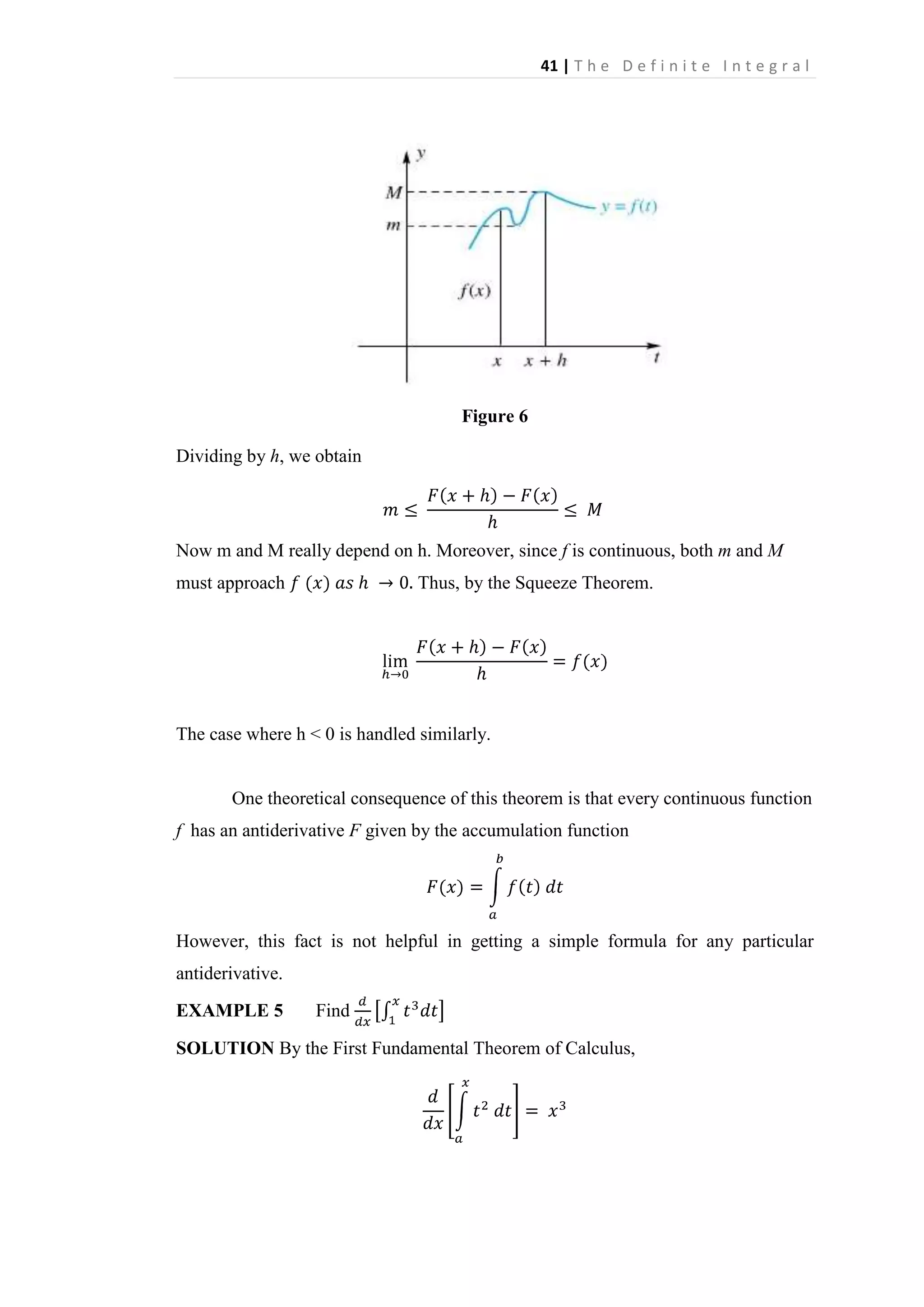
The picture in Figure 6 helps us to understand the theorem. Note that m(b — a) is the
area of the lower, small rectangle. M (b — a) is the area of the large rectangle, and
is the area under the curve.
To prove the right-hand inequality, let
for all x in [a,b]. Then, by
Theorem 3.4,
However,
is aqual to the area of a rectangle with wideth b-a and height
M. Thus.
The left-hand inequality is handled similarly.
The Definite Integral is a Linear Operator
Earlier we learned that
and
linear operators. You can add
to the list.
Theorem 3.5 Linearity of the Definite Integral
Suppose that f and g are integrable on [a,b] and that k is a constant. Then kf
f + g are integrable and
and

33. 40 | T h e D e f i n i t e I n t e g r a l
(i)
(ii)
(iii)
Proof The proofs of (i) and (ii) depend on the linearity of and the properties of limits.
We show (ii).
Part (iii) follows from (i) and (ii) on writing
Proof of the First Fundamental Theorem of Calculus With these results in hand,
we are now ready to prove the First Fundamental Theorem of Calculus.
Proof In the sketch of the proof presented earlier. we defined
and we established the fact that
Assume. for the moment that h > 0 and let m and M be the minimum value
and maximum value., respectively, of f on the interval [x,x + h] (Figure 6). By
Theorem 3.5 ,
or

34. 41 | T h e D e f i n i t e I n t e g r a l
Figure 6
Dividing by h, we obtain
Now m and M really depend on h. Moreover, since f is continuous, both m and M
must approach
Thus, by the Squeeze Theorem.
The case where h < 0 is handled similarly.
One theoretical consequence of this theorem is that every continuous function
f has an antiderivative F given by the accumulation function
However, this fact is not helpful in getting a simple formula for any particular
antiderivative.
EXAMPLE 5
Find
SOLUTION By the First Fundamental Theorem of Calculus,

35. 42 | T h e D e f i n i t e I n t e g r a l
EXAMPLE 6
Find
SOLUTION We challenge anyone to do this example by first evaluating the
integral. However, by the. First Fundamental Theorem of Calculus, it is a trivial
problem.
EXAMPLE 7
Find
.
SOLUTION Use of the dummy variable rather than t should not bother anyone.
However, the fact that x is the lower limit, rather than the upper limit, is troublesome.
Here. is how we handle this difficulty.
The interchange of the upper and lower limits is allowed if we prefix a negative sign.
(Recall that by definition
EXAMPLE 8
Find
in two ways
SOLUTION One way to find this derivative is to apply the First Fundamental
Ilieorem of Calculus, although riow we have a new complication:, the upper limit is
rather than x. This problem is handled by the Chain Rule. We may think of the
expression in brackets as
By the Chain Rule, the derivative with respect to x of this composite function is

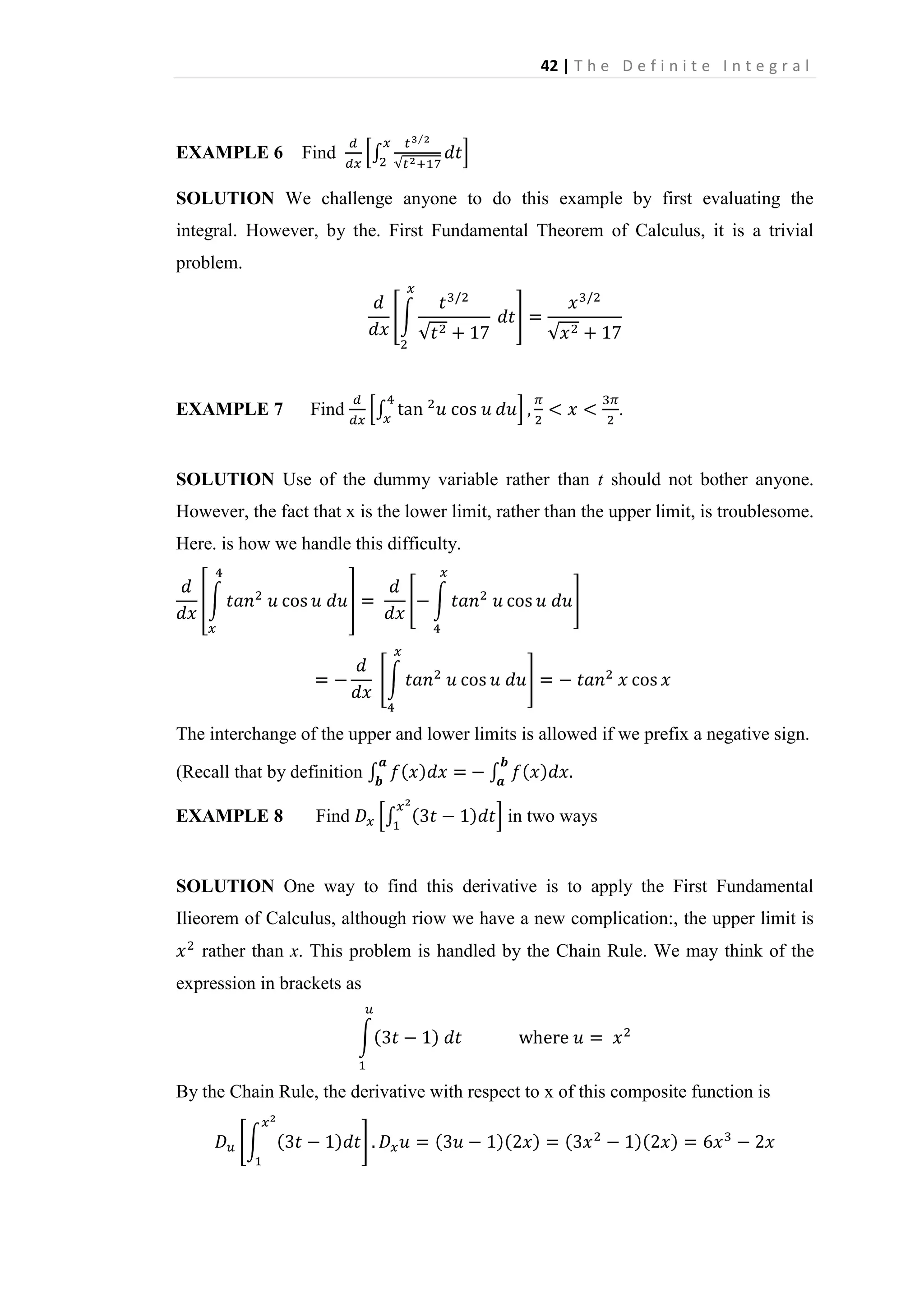
36. 43 | T h e D e f i n i t e I n t e g r a l
Another way to find this derivative is to evaluate the definite integral first and
then use our rules for derivatives. The definite integral
below the tine y = 3t – 1 between t = 1 and t =
–
is the area
(see. Figure 7). Since. the area of
this trapezoid is
Thua ,
Position as Accumulated Velocity In the last section we saw how the position of an
object, initially at the origin, is equa[ to the definite integral of the velocity function,
This often leads to accumulation functions, as the next example illustrates.
2.4 The Second Fundamental Theorem of Calculus and Method of Subtitution
The First Fundamental Theorem of Calculus, given in the previous section, gives the
inverse relationship between definite integrals and derivatives. Although it is not yet
apparent, this relationship gives us a powerful tool for evaluating definite integrals.
This tool is called the Second Fundamental Theorem of Calculus, and we will apply
it much more often than the First Fundamental Theorem of Calculus.
Theorem 3.6 Second Fundamental Theorem of Calculus
Let f be continuous (hence integrable) on [a, b], and let F be any antiderivative of f
on [a, b]. Then
Proof For x in the interval [a, b] define
. Then, by the First
Fundamental Theorem of Calculus, G' (x) = f(x) for all in (a, b). Thus. G is an
antiderivative off; but F is also an antiderivative of f, we conclude that since F'(x)=
G'(x), the functions F and G differ by a constant. Thus, for all x in (a, b)
F(x) = G(x) + C

37. 44 | T h e D e f i n i t e I n t e g r a l
Since the function F and G are continuous on the closed interval [a,b], we have F(a)
= G(a) + C and F(b)=G(b) + C. Thus, F(x) = G(x) + C on the closed interval [a,b].
Since
, we have
Therefore,
EXAMPLE 9 Show that
SOLUTION
, where k is a constant.
is an antiderivative of f (x) = k. Thus, by the Second
Fundamental Theorem of Calculus,
.
EXAMPLE 10 Show that
SOLUTION
.
is an antiderivative
. Therefore,
.
EXAMPLE 11 Show that if r is a rational number different from -1. Then
SOLUTION
is an antiderivative of
. Thus, by the Second
Fundamental Theorem of Calculus.
If r < 0, we require that 0 not be in [a, b]. Why?
It is convenient to introduce a special symbol for F(b) - F (a). We write
With this notation,
.

38. 45 | T h e D e f i n i t e I n t e g r a l
EXAMPLE 12 Evaluate
SOLUTION
.
Theorem 3.7 Substitution Rule for Indefinite Integrals
Let g be a differentiable function and suppose that F is an antiderivative of f. Then
Proof All we need to do to prove this result is to show that the derivative of the right
side is equal to the integrand of the integral on the left_This is a simple application of
the Chain Rule.
We normally apply Theorem 3.7 as follows. In an integral such as
, we let u = g(x), so that
Thus, du = g' (x) dx.
The integral then becomes
Thus, if we can find an antiderivative for f (x), we can evaluate
The trick to applying the method of substitution is to choose the right substitution to
make. In some cases this substitution is obvious; in other cases it is not so obvious.
Proficiency in applying the method of substitution comes from practice.
EXAMPLE 13 Evaluate
SOLUTION
.
The obvious substitution here is u = 3x, so that du = 3 dx. Thus
.

39. 46 | T h e D e f i n i t e I n t e g r a l
Notice how we had to multiply by . 3 in order to have the expression 3dx = du in
the integral.
EXAMPLE 14 Evaluate
SOLUTION
.
Here the appropriate substitution is
. This gives us
in the integrand, but more importantly, the extra x in the integrand can be put
with the differential, because du = 2x dx. Thus
.
EXAMPLE 15 Evaluate
SOLUTION
Let
.
; then
. Thus,
Therefore, by the Second Fundamental Theorem of Calculus,
Theorem 3.7 Substitution Rule for Definite Integrals
Let g have a continuous derivative on [a, b], and let f be continuous on the range of
g. Then
where
.
Proof Let F be an antiderivative of f . Then, by the Second Fundamental Theorem
of Calculus,
On the other hand, by the Substitution Rule for Indefinite Integrals

40. 47 | T h e D e f i n i t e I n t e g r a l
and so, again by the Second Fundamental Theorem of Calculus,
.
EXAMPLE 16 Evaluate
SOLUTION Let
.
, so
, and note that
when x = 0 and u = 9 when x = 1. Thus,
Exercises 2.4
In Problems 1 - 5, use the Second Fundamental Theorem of Calculus to evaluate
each definite integral.
1.
2.
3.
4.
5.
In Problem 6 – 10, use the method subtitition to find each of the following indefinite
integrals.
6.
7.
8.
9.
10.

41. 48 | T h e D e f i n i t e I n t e g r a l