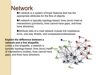
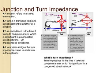
Junctions are points where links (road segments) meet in a network. Turn impedance refers to the additional cost or time needed to make a turn at a junction from one link onto another. This turn cost is an attribute typically assigned to turns in a network dataset.

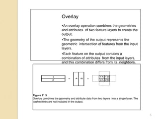
![Overlay Methods
All overlay methods are based on the Boolean connectors of AND, OR, and XOR.
An overlay operation is called Intersect if it uses the AND connector.
An overlay operation is called Union if it uses the OR connector.
An overlay operation that uses the XOR connector is called Symmetrical Difference
or Difference.
An overlay operation is called Identity or Minus if it uses the following expression:
[(input layer) AND (identity layer)] OR (input layer).
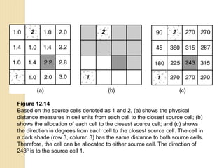
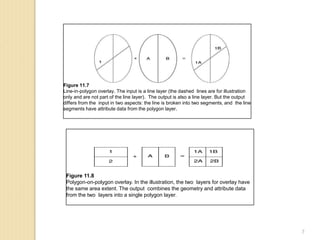
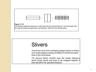
Figure 11.9
The Union method keeps all areas of the two input layers in the output.
8](https://image.slidesharecdn.com/gis-unit4-220309044327/85/Geographic-Information-System-unit-4-8-320.jpg)
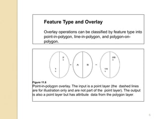
![Areal Interpolation
One common application of overlay is to help solve the areal
interpolation problem. Areal interpolation involves transferring known
data from one set of polygons (source polygons) to another (target
polygons).
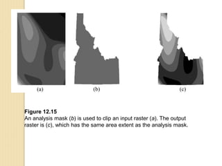
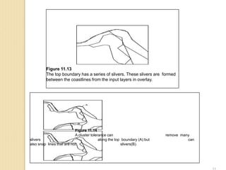
Figure 11.15
An example of areal interpolation. Thick lines represent census tracts and thin lines
school districts. Census tract A has a known population of 4000 and B has 2000. The
overlay result shows that the areal proportion of census tract A in school district 1 is
1/8 and the areal proportion of census tract B, 1/2. Therefore, the population in
school district 1 can be estimated to be 1500, or [(4000 x 1/8) + (2000 x 1/2)].
12](https://image.slidesharecdn.com/gis-unit4-220309044327/85/Geographic-Information-System-unit-4-12-320.jpg)