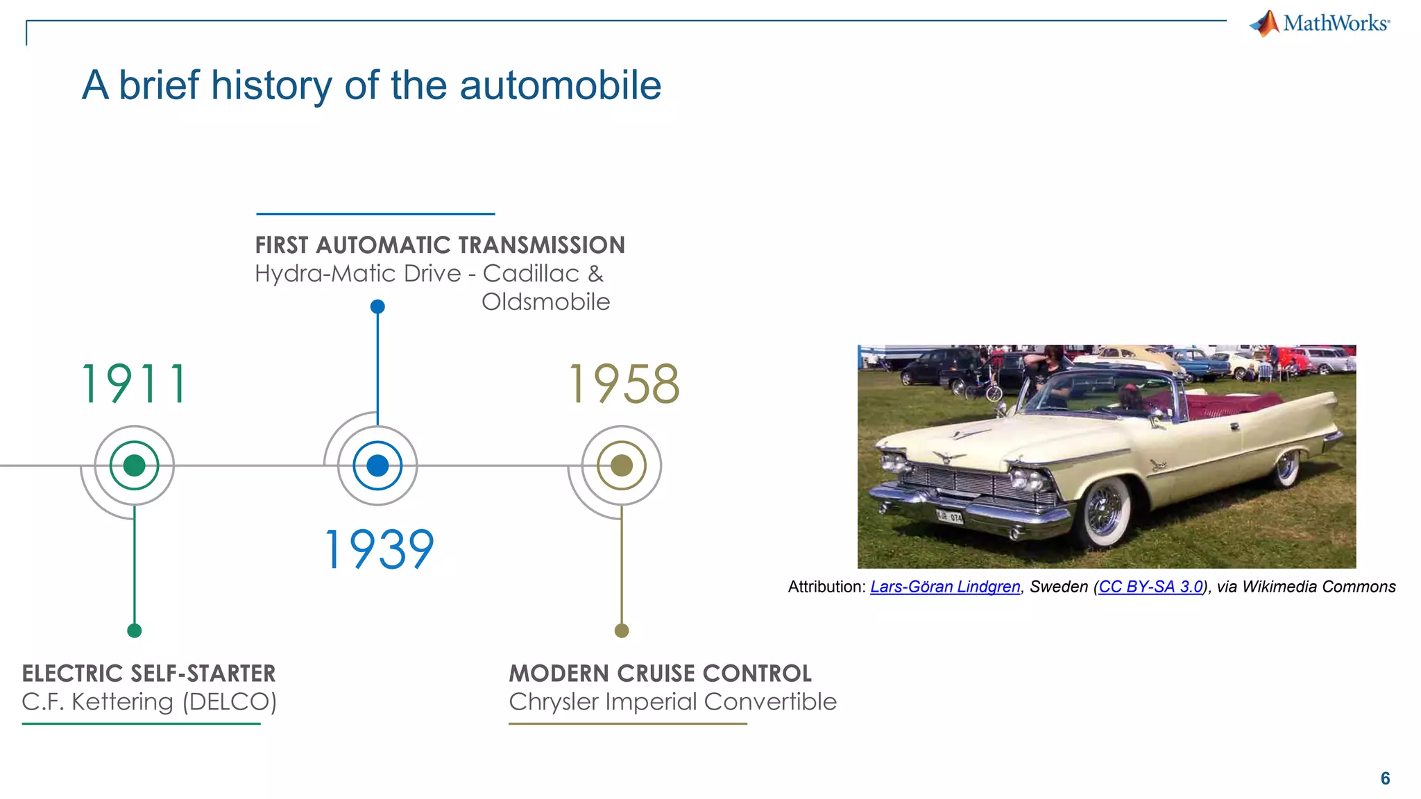
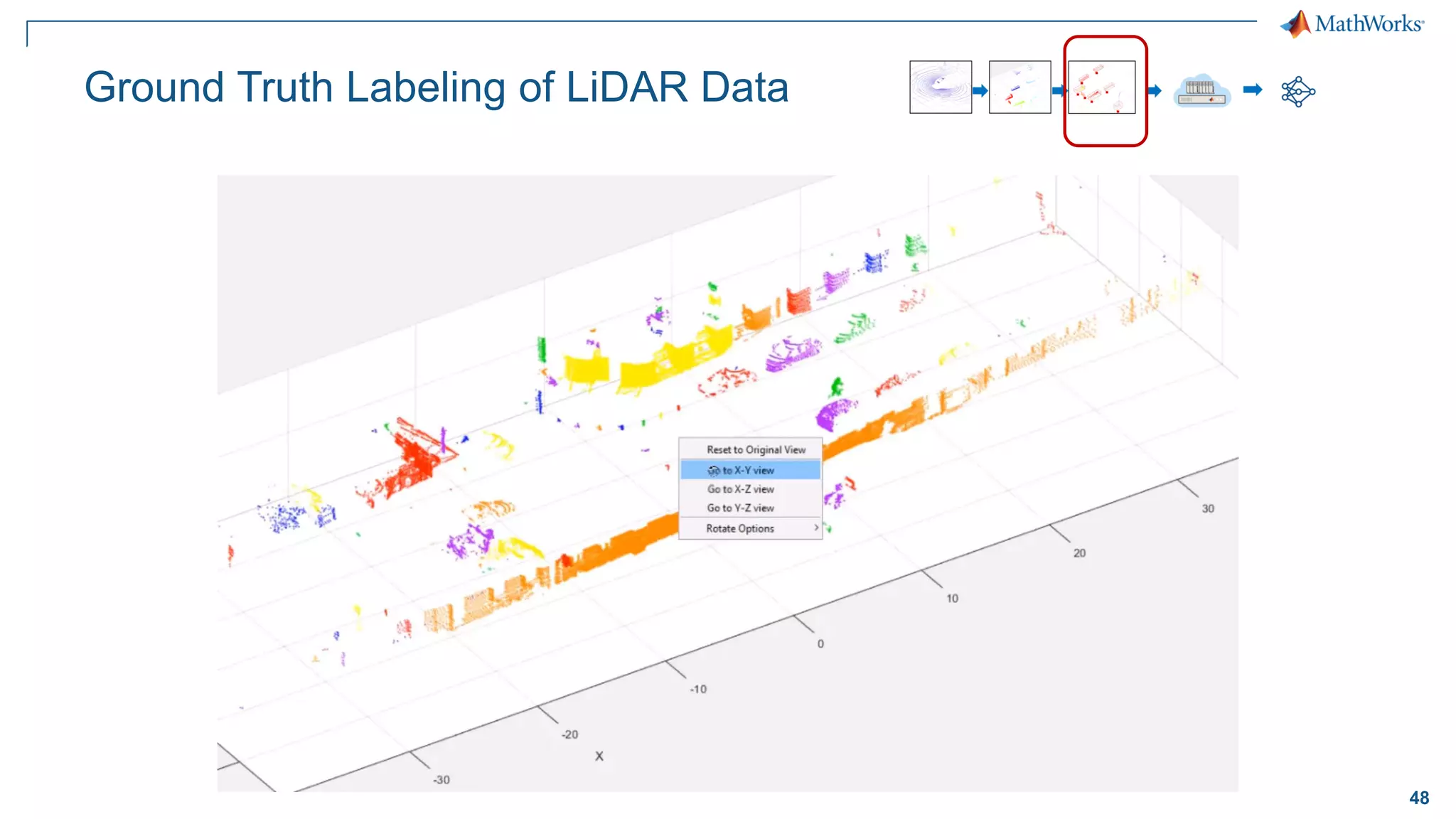
1© 2018 The MathWorks, Inc.
Deep Learning and the technology behind
Self-Driving Cars
Lucas García, PhD
Senior Application Engineer
lucas.garcia@mathworks.es
2
A brief history of the automobile
Attribution: DaimlerChrysler AG (CC-BY-SA-3.0),via Wikimedia Commons
1885
FIRST COMMERCIAL GAS CAR
Benz Patent-Motorwagen
3
1885
FIRST COMMERCIAL GAS CAR
Benz Patent-Motorwagen
A brief history of the automobile
1908
FIRST MASS PRODUCED CAR
Ford Model T
Attribution: Harry Shipler (Public domain), via Wikimedia Commons
4
1885
FIRST COMMERCIAL GAS CAR
Benz Patent-Motorwagen
A brief history of the automobile
1908
FIRST MASS PRODUCED CAR
Ford Model T
1911
ELECTRIC SELF-STARTER
C.F. Kettering (DELCO) Attribution: Charles F. Kettering, U.S. Patent 1,150,523
5
1911
ELECTRIC SELF-STARTER
C.F. Kettering (DELCO)
A brief history of the automobile
1939
FIRST AUTOMATIC TRANSMISSION
Hydra-Matic Drive - Cadillac &
Oldsmobile
Attribution: Michael Barera (CC BY-SA 4.0),via Wikimedia Commons
6
1911
ELECTRIC SELF-STARTER
C.F. Kettering (DELCO)
A brief history of the automobile
1939
FIRST AUTOMATIC TRANSMISSION
Hydra-Matic Drive - Cadillac &
Oldsmobile
1958
MODERN CRUISE CONTROL
Chrysler Imperial Convertible
Attribution: Lars-Göran Lindgren, Sweden (CC BY-SA 3.0), via Wikimedia Commons
7
1911
ELECTRIC SELF-STARTER
C.F. Kettering (DELCO)
A brief history of the automobile
1939
FIRST AUTOMATIC TRANSMISSION
Hydra-Matic Drive - Cadillac &
Oldsmobile
1958
MODERN CRUISE CONTROL
Chrysler Imperial Convertible
1971
ANTI-LOCK BRAKING SYSTEM
“Sure-Brake”, First Computerized ABS
Attribution: Chris828 (Public domain),
via Wikimedia Commons
8
A brief history of the automobile
1971
ANTI-LOCK BRAKING SYSTEM
“Sure-Brake”, First Computerized ABS
1981
FIRST ECU
General Motors, Motorola
9
A brief history of the automobile
1971
ANTI-LOCK BRAKING SYSTEM
“Sure-Brake”, First Computerized ABS
1981
FIRST ECU
General Motors, Motorola
1996
FIRST CONNECTED CAR
OnStar
Attribution: Tyler from Riverside, USA (CC BY 2.0), via Wikimedia Commons
10
A brief history of the automobile
1971
ANTI-LOCK BRAKING SYSTEM
“Sure-Brake”, First Computerized ABS
1981
FIRST ECU
General Motors, Motorola
1996
FIRST CONNECTED CAR
OnStar
2000
LANE DEPARTURE WARNING SYSTEM
Mercedes-Benz Actros
11
A brief history of the automobile
1971
ANTI-LOCK BRAKING SYSTEM
“Sure-Brake”, First Computerized ABS
1981
FIRST ECU
General Motors, Motorola
1996
FIRST CONNECTED CAR
OnStar
2000
LANE DEPARTURE WARNING SYSTEM
Mercedes-Benz Actros
12
A brief history of the automobile
13
Localization and PlanningLocalization and Planning
Perception Control
Most prominent areas in automated driving
ControlPerception
Deep learning
Path planning
Sensor models &
model predictive control
Sensor fusion
14
Perception Control
Localization and Planning
Focus of today’s presentation
Perception
Deep learning
Sensor fusion
Sensor models &
model predictive control
Path planning
15
Shallow Machine Learning vs. Deep Learning
Shallow Machine Learning
Deep Learning
Deep Learning learns
both features and tasks
directly from data
Machine Learning learns
tasks using features
extracted manually from data
End-to-End Learning
16
▪ Train “deep” neural networks on structured data (e.g. images, signals, text)
▪ Implements Feature Learning: Eliminates need for “hand crafted” features
▪ Trained using GPUs for performance
Convolutional Neural Networks
Convolution +
ReLu PoolingInput
Convolution +
ReLu Pooling
…
…
Flatten Fully
Connected
Softmax
car
truck
bicycle
…
van
…
…
Feature Learning Classification
17
Deep Learning Workflow
Select Network
Architecture
Build from scratch
Interoperability
Use/tune pretrained
networks
3
Images
Signals
Text
Access and Explore Data
1
Share and Deploy
Share and export
Enterprise Scale
Systems
Embedded Devices
and Hardware
5
Perform Training
CPU vs. GPU
Hyperparameter
tuning
Scale training
4
Label and
Preprocess Data
Label training data
Data augmentation
Synthetic Data
2
18
Automate Labeling with Ground-Truth Labeler App
Learn more
19
Automate Labeling with Ground-Truth Labeler App
Learn more
20
Original Image
ROI detection
Pixel classification
ROI detection vs. Pixel classification
21
Pixel Labeling
22
Semantic Segmentation Network
Boat
Airplane
Other classes
23
Semantic Segmentation Network
24
Semantic Segmentation
CamVid Dataset
1. Segmentation and Recognition Using Structure from Motion Point Clouds, ECCV 2008
2. Semantic Object Classes in Video: A High-Definition Ground Truth Database, Pattern Recognition Letters
25
Load and plot training images
% Create datastore for images
imds = imageDatastore(imgDir);
I = readimage(imds, 1);
I = histeq(I);
imshow(I)
imageDatastore
manages large collections
of images
26
Load and overlay pixel labels
% Load pixel labels
classes = ["Sky"; "Building";...
"Pole"; "Road"; "Pavement"; "Tree";...
"SignSymbol"; "Fence"; "Car";...
"Pedestrian"; "Bicyclist"];
pxds = pixelLabelDatastore(...
labelDir,classes,labelIDs);
% Display labeled image
C = readimage(pxds, 1);
cmap = camvidColorMap;
B = labeloverlay(I,C,'ColorMap',cmap);
imshow(B)
pixelLabelDatastore
manages large collections
of pixel labels
27
Visualize distribution of labeled pixels
% Visualize label count by class
tbl = countEachLabel(pxds)
frequency = tbl.PixelCount / ...
sum(tbl.PixelCount);
bar(1:numel(classes),frequency)
xticks(1:numel(classes))
xticklabels(tbl.Name)
xtickangle(45)
ylabel('Frequency')
Likely to
detect roads
Unlikely to
detect
bicyclist
Labeled pixels in this set are
imbalanced
28
Create and visualize baseline network
% Create SegNet architecture
lgraph = segnetLayers(...
imageSize, numClasses,...
'vgg16');
% Display network structure
plot(lgraph)
title('Complete Layer Graph')
% Display last layers
plot(lgraph);
title('Last 9 Layers Graph')
Last
network layer
29
Last
network layer
Compensate for imbalanced data set
% Create weighted layer
pxLayer = pixelClassificationLayer(...
'Name', 'weightedLabels', ...
'ClassNames', tbl.Name, ...
'ClassWeights', classWeights)
30
Last
network layer
Compensate for imbalanced data set
% Create weighted layer
pxLayer = pixelClassificationLayer(...
'Name', 'weightedLabels', ...
'ClassNames', tbl.Name, ...
'ClassWeights', classWeights)
% Replace layer
lgraph = removeLayers(lgraph, 'pixelLabels');
lgraph = addLayers(lgraph, pxLayer);
lgraph = connectLayers(lgraph,...
'softmax', 'weightedLabels');
% Display network structure
plot(lgraph);
title('Replaced Layers Graph')
31
Augment images to expand training set
augmenter = imageDataAugmenter(...
'RandXReflection', true,...
'RandRotation', [-30 30],... % degrees
'RandXTranslation', [-10 10],... % pixels
'RandYTranslation', [-10 10]); % pixels
datasource = pixelLabelImageSource(...
imdsTrain, ... % Image datastore
pxdsTrain, ... % Pixel datastore
'DataAugmentation', augmenter)
32
options = trainingOptions('sgdm', ...
'Momentum', 0.9, ...
'InitialLearnRate', 1e-2, ...
'L2Regularization', 0.0005, ...
'MaxEpochs', 120, ...
'MiniBatchSize', 4, ...
'Shuffle', 'every-epoch', ...
'Verbose', false, ...
'ExecutionEnvironment', 'auto', ...
'Plots','training-progress');
Deep learning on CPU, GPU, multi-GPU and clusters
Single CPU Single CPU
Single GPU
Single CPU
Multiple GPUs
On-prem server with
GPUs
Cloud GPUs
(AWS, Azure, etc.)
33
Train network and view progress
[net, info] = trainNetwork(datasource, lgraph, options);
34
Evaluate trained network on image
% Plot actual results
I = read(imdsTest);
actual = semanticseg(I, net);
B = labeloverlay(I, ...
actual,...
'Colormap', cmap,...
'Transparency',0.4);
imshow(B)
pixelLabelColorbar(cmap, classes);
title('Actual')
35
Visually compare actual with original labeled results
% Plot expected results
% using original labels
expected = read(pxdsTest);
E = labeloverlay(I,...
expected,...
'Colormap', cmap,...
'Transparency', 0.4);
imshow(E)
title('Expected');
36
Visually compare actual with original labeled results
% Plot differences
imshowpair(...
uint8(actual),...
uint8(expected));
title('Difference');
37
Assess similarity using intersection-over-union (IoU) metric
iou = jaccard(actual,...
expected);
table(classes, iou)
ans =
11×2 table
classes iou
____________ ________
"Sky" 0.92659
"Building" 0.7987
"Pole" 0.16978
"Road" 0.95177
"Pavement" 0.41877
"Tree" 0.43401
"SignSymbol" 0.32509
"Fence" 0.492
"Car" 0.068756
"Pedestrian" 0
"Bicyclist" 0
38
Evaluate trained network statistics
pxdsResults = ...
semanticseg(...
imdsTest,net,...
'WriteLocation', tempdir,...
'Verbose', false);
metrics = ...
evaluateSemanticSegmentation(...
pxdsResults, pxdsTest,...
'Verbose', false);
metrics.ClassMetrics
Evaluation metrics of network
39
Distribution of labels in data affects intersection-over-union (IoU)
Underrepresented classes such as Pedestrian and Bicyclist are
not segmented as well as classes such as Sky and Road
Distribution of labels in original data set Evaluation metrics of network
40
Radar
Sensors
Ultrasonic LiDAR
Passive Visual
Charts credit: cleantechnica.com
41
Sensor Fusion
Charts credit: cleantechnica.com
42
Light Detection and Ranging - LiDAR
LiDAR
Attribution: Steve Jurvetson - derivative work: Mariordo (CC BY 2.0), via Wikimedia Commons
43
What does LiDAR Data look like?
44
Data preparation and labeling of LiDAR is a challenge
Trained
DNN
DNN
design + training
Accessing
LiDAR data
TrainingLiDAR pre-
processing
Labeling
LiDAR data
45
Access and Visualize LiDAR Data
Access Stored Lidar Data
▪ Velodyne file I/O (pcap)
▪ Individual point clouds (.pcd,ply)
▪ Custom binary formats
Visualize Lidar Data
▪ Streaming LiDAR player
▪ Static point cloud display
▪ Point cloud differences
46
Lidar Preprocessing
Remove Ground
• Fit plane using RANSAC
• segmentGroundFromLidarData
Cluster
• Segment clusters using
Euclidean distance
• segmentLidarData
47
Ground Truth Labeling of LiDAR Data
48
Ground Truth Labeling of LiDAR Data
49
Ground Truth Labeling of LiDAR Data
50
Option #1: Classify Individual Point Clouds
Reference: PointNet: Deep Learning on Point Sets for 3D Classification and Segmentation
51
PointNet Network Structure
Reference: PointNet: Deep Learning on Point Sets for 3D Classification and Segmentation
52
Applying Deep Classifier to clusters
>> classify(net, pts)
53
Option #2: LiDAR Semantic Segmentation (using LinkNet)
Cars
Trucks
Ground
54
Organize Data for Training
Raw Point Cloud Data
Ground Truth Labels Transformed to Label Mask
Project to 2D
55
Create LinkNet Semantic Segmentation
Architecture
Reference: LinkNet: Exploiting Encoder Representations for Efficient Semantic Segmentation
Easy MATLAB API
to create network
%build encoder
nOutputs = 64;
inputLayerName = 'init_maxpool';
for blockIdx = 1:encoderDepth
[lGraph, layerOutName] = encoderBlock(lGraph, blockIdx, nOutputs, inputLayerName);
nOutputs = nOutputs * 2;
inputLayerName = layerOutName;
end
%build decoder
nInputs = nOutputs;
inputLayerName = layerOutName;
for blockIdx = encoderDepth:-1:1
nOutputs = min(nInputs/2, 64);
[lGraph, decoderLayerOutName] = decoderBlock(lGraph, blockIdx, nInputs, nOutputs, inputLayerName);
if blockIdx ~= 1
inputLayerName = ['res_add' num2str(blockIdx)];
lGraph = addLayers(lGraph, additionLayer(2, 'Name', inputLayerName) );
lGraph = connectLayers(lGraph, ['enc' num2str(blockIdx-1) '_addout'], [inputLayerName '/in2']);
lGraph = connectLayers(lGraph, decoderLayerOutName, [inputLayerName '/in1']);
end
nInputs = nInputs/2;
end
56
Training LinkNet Semantic Segmentation
Train Semantic SegmentationLinkNet uses ResNet-18 Encoder/Decoder
57
Deployment using GPU Coder
C++/CUDA
+ TensorRT
C++/CUDA
+ cuDNN
58
ResNet-50 Inference on NVIDIA Titan V
MATLAB GPU Coder +
TensorRT 4 (int8)
MATLAB GPU Coder +
TensorRT 4
MATLAB GPU Coder + cuDNN
PyTorch
TensorFlow
Batch Size
Framespersecond
Testing platform
CPU: Intel Xeon CPU E5 -1650 v3 @ 3.5 GHz
GPU: NVIDIA Titan-V
59
ResNet-50 Inference on NVIDIA Titan V
Batch Size
Framespersecond
Testing platform
CPU: Intel Xeon CPU E5 -1650 v3 @ 3.5 GHz
GPU: NVIDIA Titan-V
MATLAB GPU Coder +
TensorRT 4 (int8)
TensorFlow +
TensorRT 4 (int8)
MATLAB GPU Coder +
TensorRT 4 (fp32)
TensorFlow +
TensorRT 4 (fp32)
60
LiDAR semantic segmentation
61
Learn more about perception applications for Deep Learning and
Automated Driving
Deep Learning Toolbox | Automated Driving System Toolbox | GPU Coder
Deep Learning
https://www.mathworks.com/deeplearning
Automated Driving
https://www.mathworks.com/adas
Visit our booth!
62© 2018 The MathWorks, Inc.
MATLAB and Simulink are registered trademarks of The MathWorks, Inc. See www.mathworks.com/trademarks for a list of additional trademarks.
Other product or brand names may be trademarks or registered trademarks of their respective holders.”

Deep Learning and the technology behind Self-Driving Cars

  • 1.
    1© 2018 TheMathWorks, Inc. Deep Learning and the technology behind Self-Driving Cars Lucas García, PhD Senior Application Engineer lucas.garcia@mathworks.es
  • 2.
    2 A brief historyof the automobile Attribution: DaimlerChrysler AG (CC-BY-SA-3.0),via Wikimedia Commons 1885 FIRST COMMERCIAL GAS CAR Benz Patent-Motorwagen
  • 3.
    3 1885 FIRST COMMERCIAL GASCAR Benz Patent-Motorwagen A brief history of the automobile 1908 FIRST MASS PRODUCED CAR Ford Model T Attribution: Harry Shipler (Public domain), via Wikimedia Commons
  • 4.
    4 1885 FIRST COMMERCIAL GASCAR Benz Patent-Motorwagen A brief history of the automobile 1908 FIRST MASS PRODUCED CAR Ford Model T 1911 ELECTRIC SELF-STARTER C.F. Kettering (DELCO) Attribution: Charles F. Kettering, U.S. Patent 1,150,523
  • 5.
    5 1911 ELECTRIC SELF-STARTER C.F. Kettering(DELCO) A brief history of the automobile 1939 FIRST AUTOMATIC TRANSMISSION Hydra-Matic Drive - Cadillac & Oldsmobile Attribution: Michael Barera (CC BY-SA 4.0),via Wikimedia Commons
  • 6.
    6 1911 ELECTRIC SELF-STARTER C.F. Kettering(DELCO) A brief history of the automobile 1939 FIRST AUTOMATIC TRANSMISSION Hydra-Matic Drive - Cadillac & Oldsmobile 1958 MODERN CRUISE CONTROL Chrysler Imperial Convertible Attribution: Lars-Göran Lindgren, Sweden (CC BY-SA 3.0), via Wikimedia Commons
  • 7.
    7 1911 ELECTRIC SELF-STARTER C.F. Kettering(DELCO) A brief history of the automobile 1939 FIRST AUTOMATIC TRANSMISSION Hydra-Matic Drive - Cadillac & Oldsmobile 1958 MODERN CRUISE CONTROL Chrysler Imperial Convertible 1971 ANTI-LOCK BRAKING SYSTEM “Sure-Brake”, First Computerized ABS Attribution: Chris828 (Public domain), via Wikimedia Commons
  • 8.
    8 A brief historyof the automobile 1971 ANTI-LOCK BRAKING SYSTEM “Sure-Brake”, First Computerized ABS 1981 FIRST ECU General Motors, Motorola
  • 9.
    9 A brief historyof the automobile 1971 ANTI-LOCK BRAKING SYSTEM “Sure-Brake”, First Computerized ABS 1981 FIRST ECU General Motors, Motorola 1996 FIRST CONNECTED CAR OnStar Attribution: Tyler from Riverside, USA (CC BY 2.0), via Wikimedia Commons
  • 10.
    10 A brief historyof the automobile 1971 ANTI-LOCK BRAKING SYSTEM “Sure-Brake”, First Computerized ABS 1981 FIRST ECU General Motors, Motorola 1996 FIRST CONNECTED CAR OnStar 2000 LANE DEPARTURE WARNING SYSTEM Mercedes-Benz Actros
  • 11.
    11 A brief historyof the automobile 1971 ANTI-LOCK BRAKING SYSTEM “Sure-Brake”, First Computerized ABS 1981 FIRST ECU General Motors, Motorola 1996 FIRST CONNECTED CAR OnStar 2000 LANE DEPARTURE WARNING SYSTEM Mercedes-Benz Actros
  • 12.
    12 A brief historyof the automobile
  • 13.
    13 Localization and PlanningLocalizationand Planning Perception Control Most prominent areas in automated driving ControlPerception Deep learning Path planning Sensor models & model predictive control Sensor fusion
  • 14.
    14 Perception Control Localization andPlanning Focus of today’s presentation Perception Deep learning Sensor fusion Sensor models & model predictive control Path planning
  • 15.
    15 Shallow Machine Learningvs. Deep Learning Shallow Machine Learning Deep Learning Deep Learning learns both features and tasks directly from data Machine Learning learns tasks using features extracted manually from data End-to-End Learning
  • 16.
    16 ▪ Train “deep”neural networks on structured data (e.g. images, signals, text) ▪ Implements Feature Learning: Eliminates need for “hand crafted” features ▪ Trained using GPUs for performance Convolutional Neural Networks Convolution + ReLu PoolingInput Convolution + ReLu Pooling … … Flatten Fully Connected Softmax car truck bicycle … van … … Feature Learning Classification
  • 17.
    17 Deep Learning Workflow SelectNetwork Architecture Build from scratch Interoperability Use/tune pretrained networks 3 Images Signals Text Access and Explore Data 1 Share and Deploy Share and export Enterprise Scale Systems Embedded Devices and Hardware 5 Perform Training CPU vs. GPU Hyperparameter tuning Scale training 4 Label and Preprocess Data Label training data Data augmentation Synthetic Data 2
  • 18.
    18 Automate Labeling withGround-Truth Labeler App Learn more
  • 19.
    19 Automate Labeling withGround-Truth Labeler App Learn more
  • 20.
    20 Original Image ROI detection Pixelclassification ROI detection vs. Pixel classification
  • 21.
  • 22.
  • 23.
  • 24.
    24 Semantic Segmentation CamVid Dataset 1.Segmentation and Recognition Using Structure from Motion Point Clouds, ECCV 2008 2. Semantic Object Classes in Video: A High-Definition Ground Truth Database, Pattern Recognition Letters
  • 25.
    25 Load and plottraining images % Create datastore for images imds = imageDatastore(imgDir); I = readimage(imds, 1); I = histeq(I); imshow(I) imageDatastore manages large collections of images
  • 26.
    26 Load and overlaypixel labels % Load pixel labels classes = ["Sky"; "Building";... "Pole"; "Road"; "Pavement"; "Tree";... "SignSymbol"; "Fence"; "Car";... "Pedestrian"; "Bicyclist"]; pxds = pixelLabelDatastore(... labelDir,classes,labelIDs); % Display labeled image C = readimage(pxds, 1); cmap = camvidColorMap; B = labeloverlay(I,C,'ColorMap',cmap); imshow(B) pixelLabelDatastore manages large collections of pixel labels
  • 27.
    27 Visualize distribution oflabeled pixels % Visualize label count by class tbl = countEachLabel(pxds) frequency = tbl.PixelCount / ... sum(tbl.PixelCount); bar(1:numel(classes),frequency) xticks(1:numel(classes)) xticklabels(tbl.Name) xtickangle(45) ylabel('Frequency') Likely to detect roads Unlikely to detect bicyclist Labeled pixels in this set are imbalanced
  • 28.
    28 Create and visualizebaseline network % Create SegNet architecture lgraph = segnetLayers(... imageSize, numClasses,... 'vgg16'); % Display network structure plot(lgraph) title('Complete Layer Graph') % Display last layers plot(lgraph); title('Last 9 Layers Graph') Last network layer
  • 29.
    29 Last network layer Compensate forimbalanced data set % Create weighted layer pxLayer = pixelClassificationLayer(... 'Name', 'weightedLabels', ... 'ClassNames', tbl.Name, ... 'ClassWeights', classWeights)
  • 30.
    30 Last network layer Compensate forimbalanced data set % Create weighted layer pxLayer = pixelClassificationLayer(... 'Name', 'weightedLabels', ... 'ClassNames', tbl.Name, ... 'ClassWeights', classWeights) % Replace layer lgraph = removeLayers(lgraph, 'pixelLabels'); lgraph = addLayers(lgraph, pxLayer); lgraph = connectLayers(lgraph,... 'softmax', 'weightedLabels'); % Display network structure plot(lgraph); title('Replaced Layers Graph')
  • 31.
    31 Augment images toexpand training set augmenter = imageDataAugmenter(... 'RandXReflection', true,... 'RandRotation', [-30 30],... % degrees 'RandXTranslation', [-10 10],... % pixels 'RandYTranslation', [-10 10]); % pixels datasource = pixelLabelImageSource(... imdsTrain, ... % Image datastore pxdsTrain, ... % Pixel datastore 'DataAugmentation', augmenter)
  • 32.
    32 options = trainingOptions('sgdm',... 'Momentum', 0.9, ... 'InitialLearnRate', 1e-2, ... 'L2Regularization', 0.0005, ... 'MaxEpochs', 120, ... 'MiniBatchSize', 4, ... 'Shuffle', 'every-epoch', ... 'Verbose', false, ... 'ExecutionEnvironment', 'auto', ... 'Plots','training-progress'); Deep learning on CPU, GPU, multi-GPU and clusters Single CPU Single CPU Single GPU Single CPU Multiple GPUs On-prem server with GPUs Cloud GPUs (AWS, Azure, etc.)
  • 33.
    33 Train network andview progress [net, info] = trainNetwork(datasource, lgraph, options);
  • 34.
    34 Evaluate trained networkon image % Plot actual results I = read(imdsTest); actual = semanticseg(I, net); B = labeloverlay(I, ... actual,... 'Colormap', cmap,... 'Transparency',0.4); imshow(B) pixelLabelColorbar(cmap, classes); title('Actual')
  • 35.
    35 Visually compare actualwith original labeled results % Plot expected results % using original labels expected = read(pxdsTest); E = labeloverlay(I,... expected,... 'Colormap', cmap,... 'Transparency', 0.4); imshow(E) title('Expected');
  • 36.
    36 Visually compare actualwith original labeled results % Plot differences imshowpair(... uint8(actual),... uint8(expected)); title('Difference');
  • 37.
    37 Assess similarity usingintersection-over-union (IoU) metric iou = jaccard(actual,... expected); table(classes, iou) ans = 11×2 table classes iou ____________ ________ "Sky" 0.92659 "Building" 0.7987 "Pole" 0.16978 "Road" 0.95177 "Pavement" 0.41877 "Tree" 0.43401 "SignSymbol" 0.32509 "Fence" 0.492 "Car" 0.068756 "Pedestrian" 0 "Bicyclist" 0
  • 38.
    38 Evaluate trained networkstatistics pxdsResults = ... semanticseg(... imdsTest,net,... 'WriteLocation', tempdir,... 'Verbose', false); metrics = ... evaluateSemanticSegmentation(... pxdsResults, pxdsTest,... 'Verbose', false); metrics.ClassMetrics Evaluation metrics of network
  • 39.
    39 Distribution of labelsin data affects intersection-over-union (IoU) Underrepresented classes such as Pedestrian and Bicyclist are not segmented as well as classes such as Sky and Road Distribution of labels in original data set Evaluation metrics of network
  • 40.
  • 41.
  • 42.
    42 Light Detection andRanging - LiDAR LiDAR Attribution: Steve Jurvetson - derivative work: Mariordo (CC BY 2.0), via Wikimedia Commons
  • 43.
    43 What does LiDARData look like?
  • 44.
    44 Data preparation andlabeling of LiDAR is a challenge Trained DNN DNN design + training Accessing LiDAR data TrainingLiDAR pre- processing Labeling LiDAR data
  • 45.
    45 Access and VisualizeLiDAR Data Access Stored Lidar Data ▪ Velodyne file I/O (pcap) ▪ Individual point clouds (.pcd,ply) ▪ Custom binary formats Visualize Lidar Data ▪ Streaming LiDAR player ▪ Static point cloud display ▪ Point cloud differences
  • 46.
    46 Lidar Preprocessing Remove Ground •Fit plane using RANSAC • segmentGroundFromLidarData Cluster • Segment clusters using Euclidean distance • segmentLidarData
  • 47.
  • 48.
  • 49.
  • 50.
    50 Option #1: ClassifyIndividual Point Clouds Reference: PointNet: Deep Learning on Point Sets for 3D Classification and Segmentation
  • 51.
    51 PointNet Network Structure Reference:PointNet: Deep Learning on Point Sets for 3D Classification and Segmentation
  • 52.
    52 Applying Deep Classifierto clusters >> classify(net, pts)
  • 53.
    53 Option #2: LiDARSemantic Segmentation (using LinkNet) Cars Trucks Ground
  • 54.
    54 Organize Data forTraining Raw Point Cloud Data Ground Truth Labels Transformed to Label Mask Project to 2D
  • 55.
    55 Create LinkNet SemanticSegmentation Architecture Reference: LinkNet: Exploiting Encoder Representations for Efficient Semantic Segmentation Easy MATLAB API to create network %build encoder nOutputs = 64; inputLayerName = 'init_maxpool'; for blockIdx = 1:encoderDepth [lGraph, layerOutName] = encoderBlock(lGraph, blockIdx, nOutputs, inputLayerName); nOutputs = nOutputs * 2; inputLayerName = layerOutName; end %build decoder nInputs = nOutputs; inputLayerName = layerOutName; for blockIdx = encoderDepth:-1:1 nOutputs = min(nInputs/2, 64); [lGraph, decoderLayerOutName] = decoderBlock(lGraph, blockIdx, nInputs, nOutputs, inputLayerName); if blockIdx ~= 1 inputLayerName = ['res_add' num2str(blockIdx)]; lGraph = addLayers(lGraph, additionLayer(2, 'Name', inputLayerName) ); lGraph = connectLayers(lGraph, ['enc' num2str(blockIdx-1) '_addout'], [inputLayerName '/in2']); lGraph = connectLayers(lGraph, decoderLayerOutName, [inputLayerName '/in1']); end nInputs = nInputs/2; end
  • 56.
    56 Training LinkNet SemanticSegmentation Train Semantic SegmentationLinkNet uses ResNet-18 Encoder/Decoder
  • 57.
    57 Deployment using GPUCoder C++/CUDA + TensorRT C++/CUDA + cuDNN
  • 58.
    58 ResNet-50 Inference onNVIDIA Titan V MATLAB GPU Coder + TensorRT 4 (int8) MATLAB GPU Coder + TensorRT 4 MATLAB GPU Coder + cuDNN PyTorch TensorFlow Batch Size Framespersecond Testing platform CPU: Intel Xeon CPU E5 -1650 v3 @ 3.5 GHz GPU: NVIDIA Titan-V
  • 59.
    59 ResNet-50 Inference onNVIDIA Titan V Batch Size Framespersecond Testing platform CPU: Intel Xeon CPU E5 -1650 v3 @ 3.5 GHz GPU: NVIDIA Titan-V MATLAB GPU Coder + TensorRT 4 (int8) TensorFlow + TensorRT 4 (int8) MATLAB GPU Coder + TensorRT 4 (fp32) TensorFlow + TensorRT 4 (fp32)
  • 60.
  • 61.
    61 Learn more aboutperception applications for Deep Learning and Automated Driving Deep Learning Toolbox | Automated Driving System Toolbox | GPU Coder Deep Learning https://www.mathworks.com/deeplearning Automated Driving https://www.mathworks.com/adas Visit our booth!
  • 62.
    62© 2018 TheMathWorks, Inc. MATLAB and Simulink are registered trademarks of The MathWorks, Inc. See www.mathworks.com/trademarks for a list of additional trademarks. Other product or brand names may be trademarks or registered trademarks of their respective holders.”