Downloaded 15 times
![Deconvolution and Interpretation of Well Test Data ‘Masked’ By Wellbore Storage in A Build…
DOI: 10.9790/5933-06521623 www.iosrjournals.org 23 | Page
Figure 3: β-deconvolved data
Figure 4: Comparison of the deconvolved and undeconvolved data
Table 5. Comparing the Undeconvolution and Deconvoluted Results
PARAMETER UNDECONVOLUTED
(MTR) MATERIAL BAL BETA'
m(psi/cycle) 70 110 200
K(mD) 8.4 5.4 3.9
S 5.87 4.2 2.7
DECONVOLUTED
References
[1]. Bassey, E.E: (1997) ‖Deconvolution of Pressure Buildup Data Distorted by Wellbore Storage and Skin in Horizontal Wells‖ M.sc
Thesis, University of Ibadan, Nigeria
[2]. Bourdet D, Ayoub, J.A and Pirard, Y.M(1998): ‖Use of pressure derivation in well test interpretation‖ SPEFE 293-302.
[3]. Horner, D.R(1951):‖Pressure Build-up in Wells‖. Proc.Third World Pet. Cong, E.J. Brill, leiden , 503-521.
[4]. Igbokoyi, A.O(2007):‖ Deconvolution of pressure buildup data distorted by wellbore storage‖ An M.sc Thesis in Petroleum
Engineering University of Ibadan, Nigeria.
[5]. kuchuk, F. J(1985):‖well testing in low transmissivity oil reservoir‖ paper SPE 13666 .SPE California Regional Meeting,
Bakersfield, March 27-29
[6]. Lee W. J:(1982)‖ Well Testing‖ New York and Dallas: Society of Petroleum Engineers of AIME
[7]. Mathew C.S and Russel, D.G(1967) ‗Pressure Build-up and flow tests in wells‘‘ Monograph Series, Society of Petroleum Engineers
of AIME, Dallas .
[8]. Oyewole, A.A(1995) :‖ Deconvolution of a two rate drawdown test distorted by wellbore storage and skin‖ M.sc Thesis, University
of Ibadan, Nigeria.
[9]. Ramey H.J Jr(1970):‖Short-time Well Test Data interpretation in the presence of skin effect and wellbore storage‖ J. Pet Tech. 97-
104
[10]. Sulaimon A(1997):‖ Deconvolution of A Two-Rate Drawdown test distorted by wellbore storage and skin‖ M.sc Thesis, University
of Ibadan, Nigeria .
[11]. Van Everdingen, A.F. and Hurst, W(1953).: ―The Application of the Laplace transformation to flow problems. Trans. AIME Vol.
186, 305-324](https://image.slidesharecdn.com/c06521623-151201072001-lva1-app6891/75/Deconvolution-and-Interpretation-of-Well-Test-Data-Masked-By-Wellbore-Storage-in-A-Build-Up-Test-8-2048.jpg)

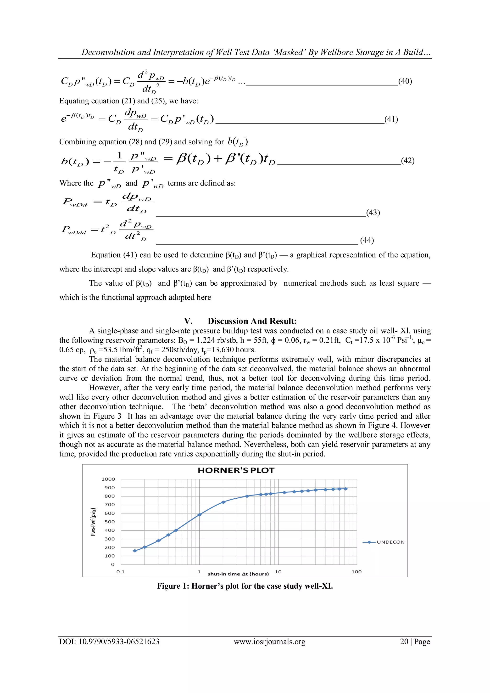
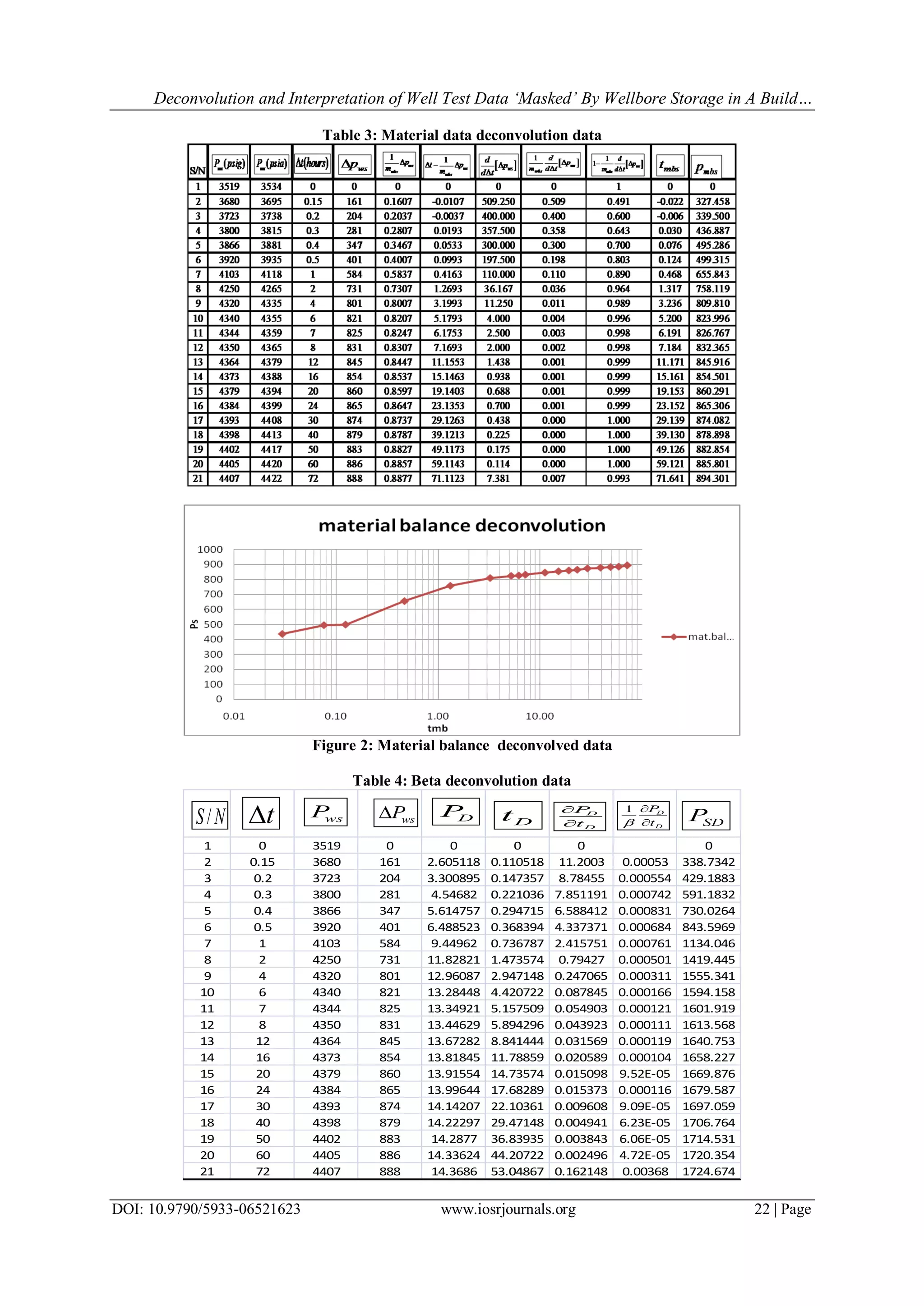
The paper discusses techniques for deconvolving well test data affected by wellbore storage during buildup tests, emphasizing the effectiveness of the material balance deconvolution method over the beta-deconvolution method for accurate reservoir parameter estimation. It compares results obtained from both methods, concluding that while the material balance technique is superior, the beta-deconvolution can still yield useful information during early testing periods. A case study demonstrates the practical application of these methods with specific reservoir parameters.


![Geotechnical Engineering-I [Lec #18: Consolidation-II]](https://cdn.slidesharecdn.com/ss_thumbnails/18-180924140946-thumbnail.jpg?width=640&height=640&fit=bounds)


![Geotechnical Engineering-I [Lec #3: Phase Relationships]](https://cdn.slidesharecdn.com/ss_thumbnails/3-180923175732-thumbnail.jpg?width=640&height=640&fit=bounds)
![Geotechnical Engineering-I [Lec #19: Consolidation-III]](https://cdn.slidesharecdn.com/ss_thumbnails/19-180924141035-thumbnail.jpg?width=640&height=640&fit=bounds)