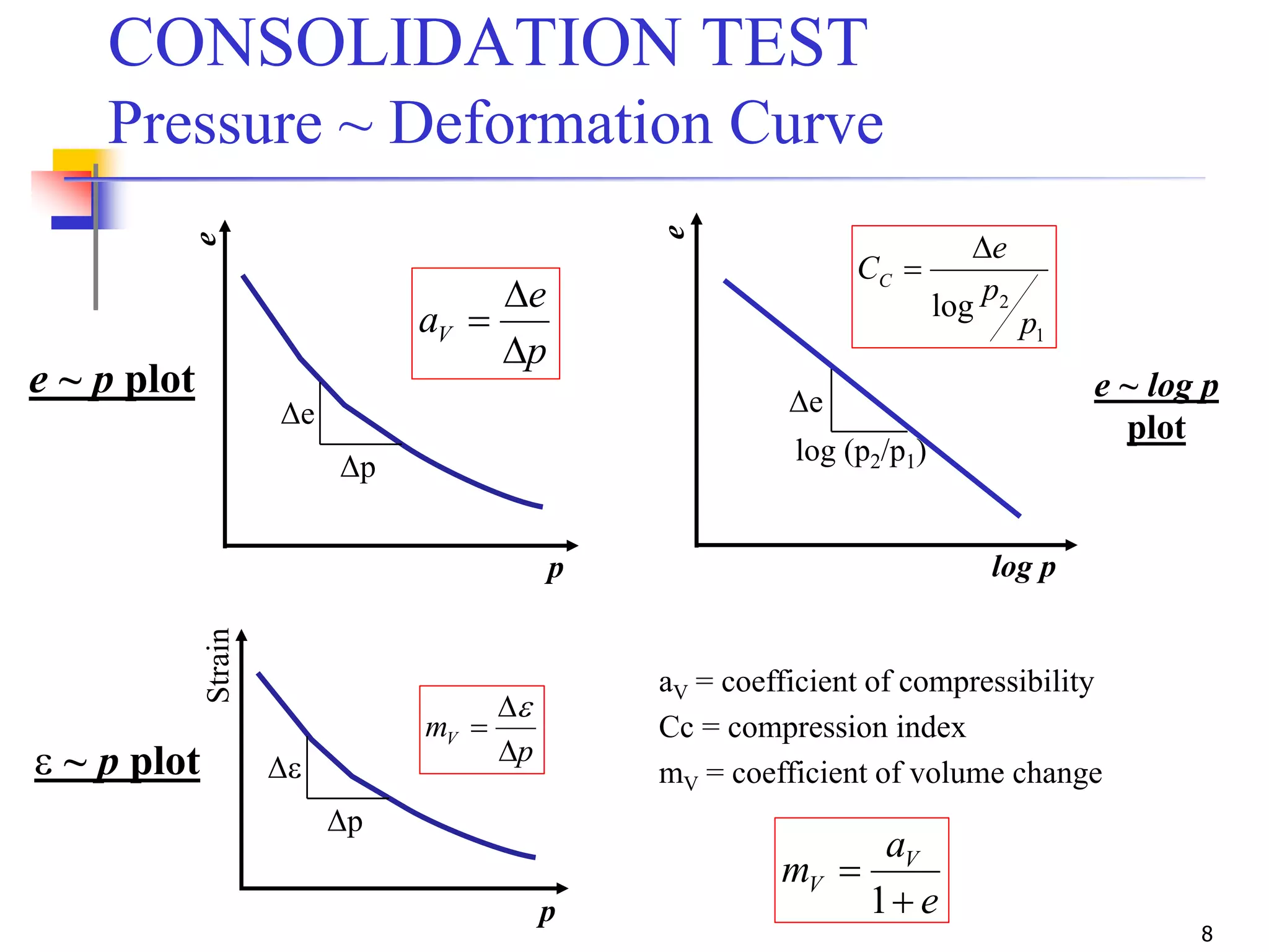
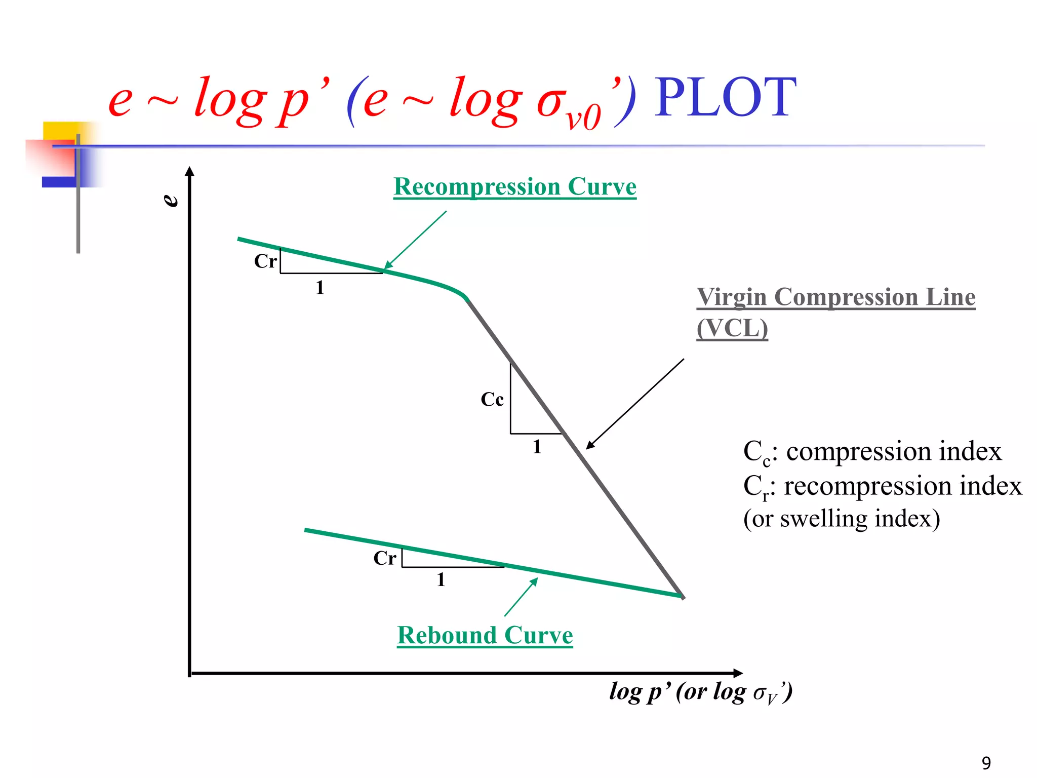
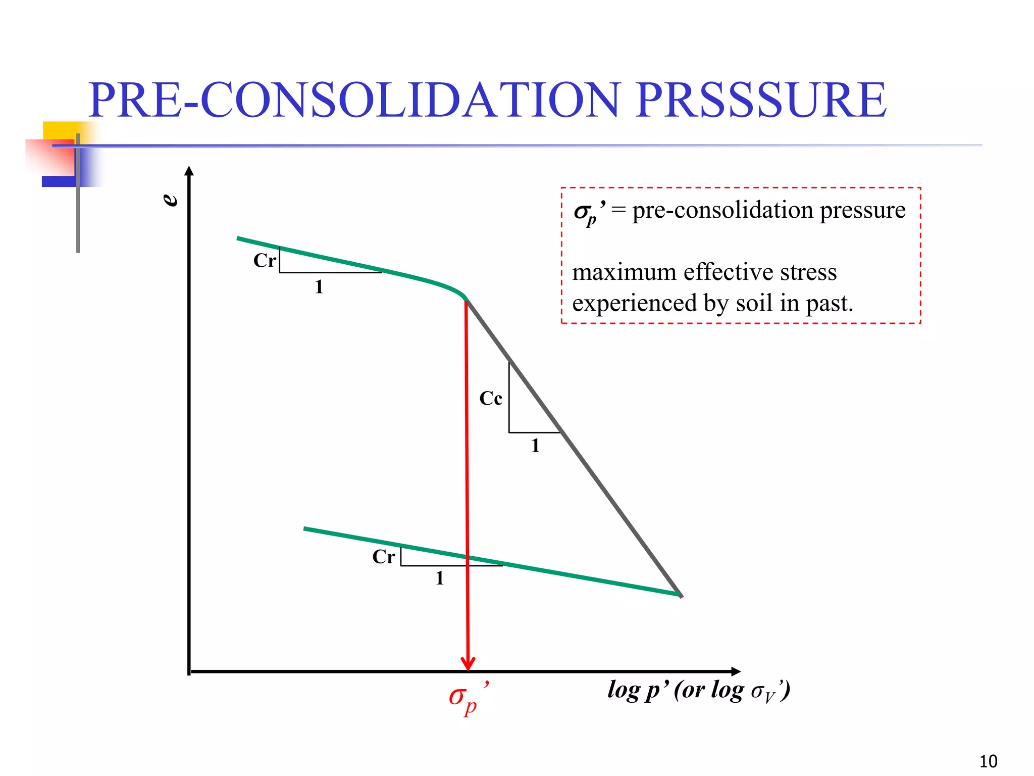
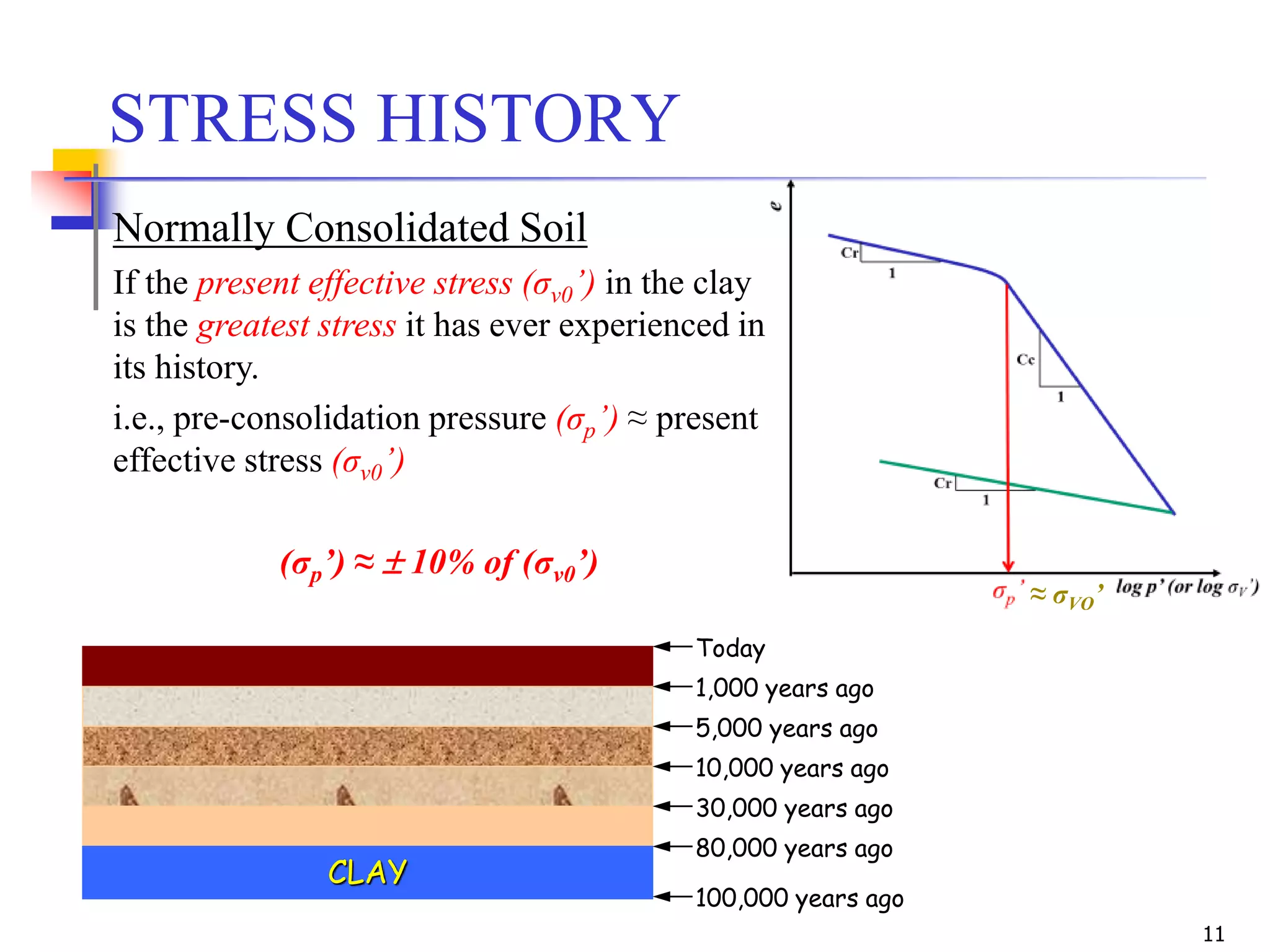
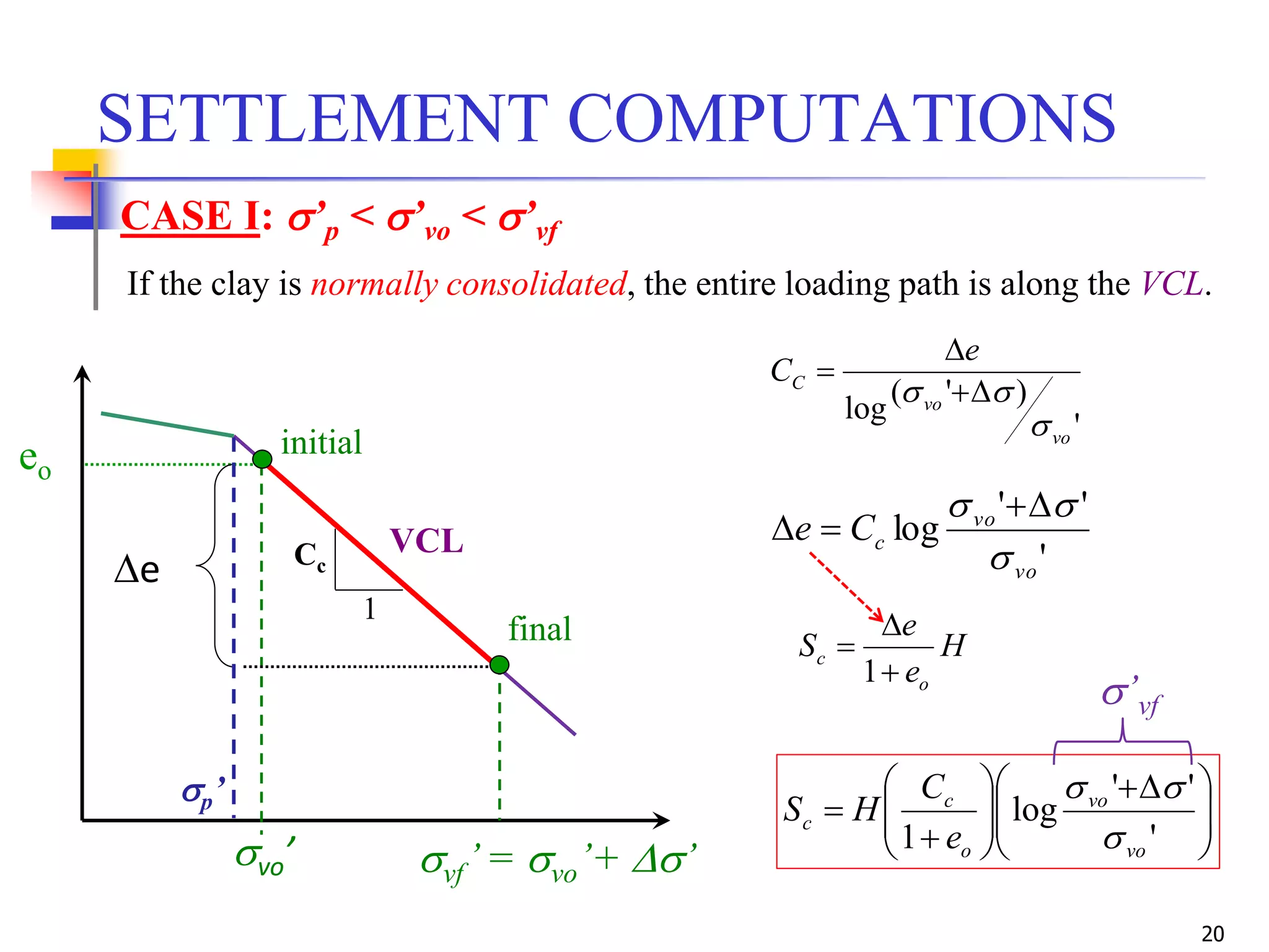
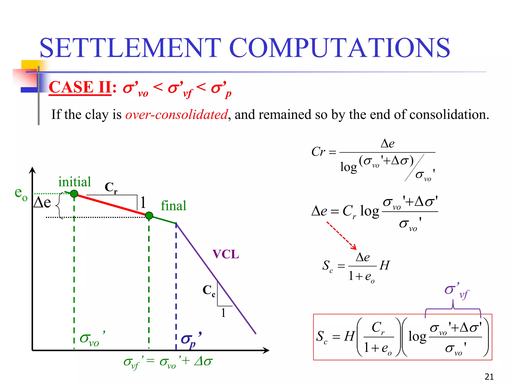
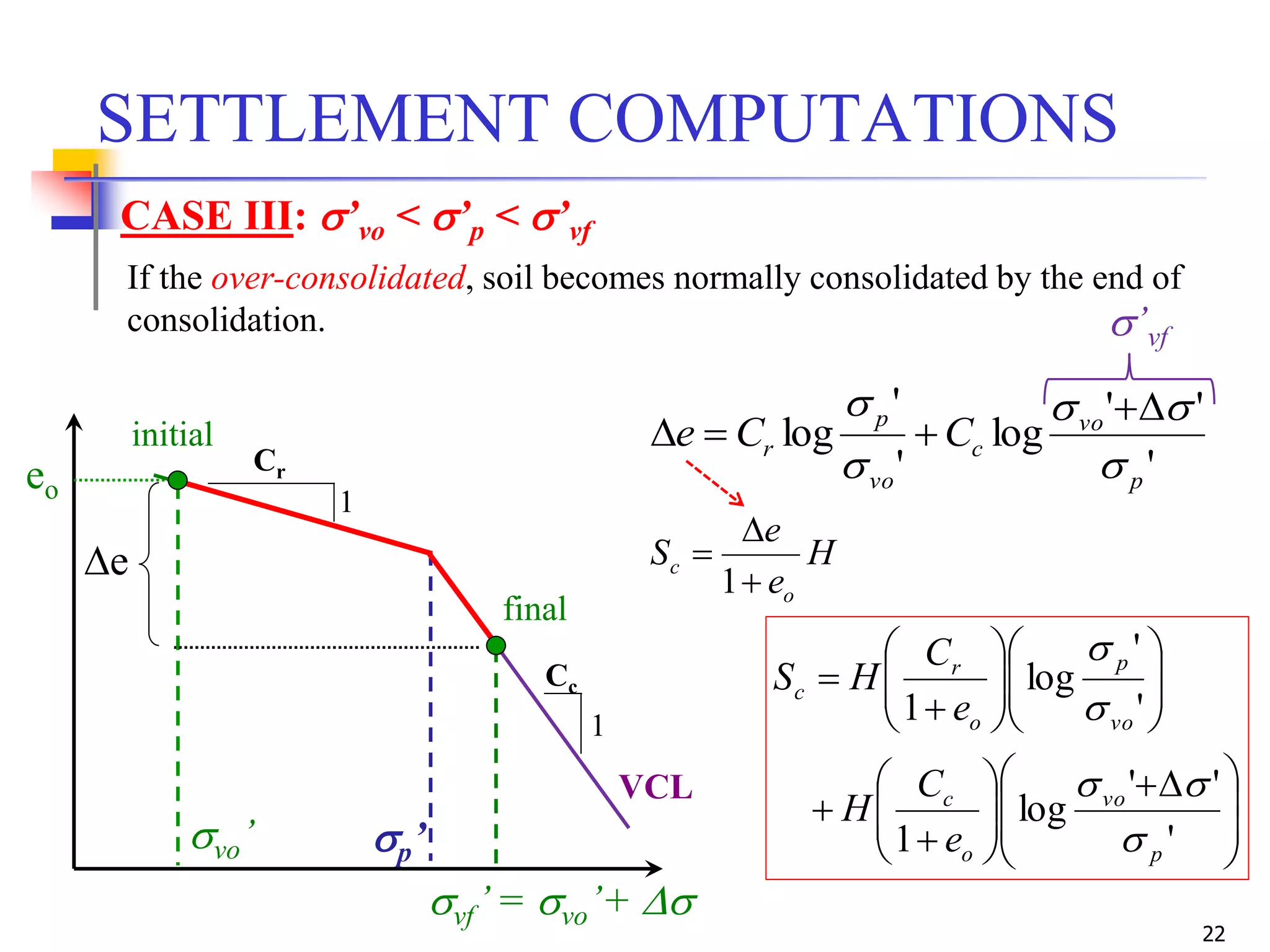
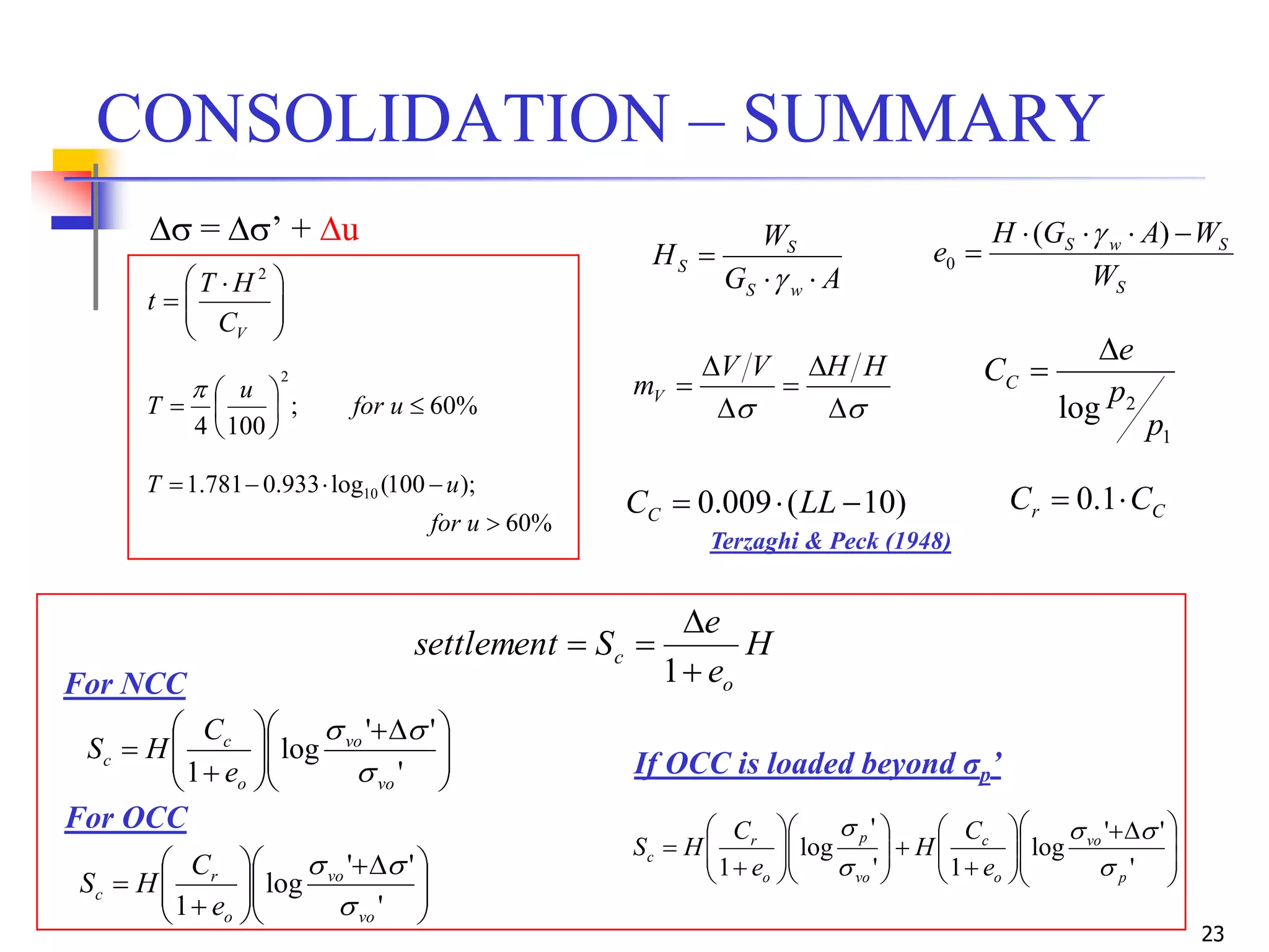
1
Geotechnical Engineering–I [CE-221]
BSc Civil Engineering – 4th Semester
by
Dr. Muhammad Irfan
Assistant Professor
Civil Engg. Dept. – UET Lahore
Email: mirfan1@msn.com
Lecture Handouts: https://groups.google.com/d/forum/2016session-geotech-i
Lecture # 19
3-Apr-2018
2
1-D Lab Consolidation
NSL
metal ring
SOIL
Porous Stones
Field
Undisturbed soil
specimen
Lab
Consolidometer / Oedometer
Stopwatch
3
CONSOLIDATION TEST
Interpretation of Test Results





 

VC
HT
t
2
Magnitude of settlement → compression index (Cc)
Rate of consolidation → co-efficient of consolidation (Cv)
Time required for consolidation (Consolidation Time) →
1. Time ~ Deformation curve
i. Cv (Coefficient of consolidation)
2. Pressure ~ Deformation curve
i. Cc (Compression index)
ii. Cr (Recompression index)
iii. aV (Coefficient of compressibility)
iv. mV (Coefficient of volume change)
SOIL
Porous
Stones
4
DEFORMATION ~ TIME PLOT
Summary
Used for determining Cv
Cv is used for determining rate of consolidation, and
consolidation time.
Casagrande’s log-time fitting method
Determines Cv corresponding to U=50%.
Deformation ~ log-time plot
Taylor’s square root of time method
Determines Cv corresponding to U=90%.
Deformation ~ square root of time plot
Cv determined from √(time) method is often slightly
greater than the log-time method.
0





 

90
2
90
t
HT
CV
5
CONSOLIDATION TEST
Pressure ~ Deformation Curve
Pressure ~ Deformation curve
i. Cc (Compression index)
ii. Cr (Recompression index)
iii. aV (Coefficient of compressibility)
iv. mV (Coefficient of volume change)
SOIL
Porous
Stones
Deformations plotted in terms of void ratio (e)
 Void ratio ~ pressure plot (e ~ p plot)
 Void ratio ~ log of pressure (e ~ log p plot)
8
CONSOLIDATION TEST
Pressure ~ Deformation Curve
p
e
aV



e ~ p plot
e
p
Δe
Δp
aV = coefficient of compressibility
Cc = compression index
mV = coefficient of volume change
Δe
log (p2/p1)
e
log p
1
2log
p
p
e
CC


e ~ log p
plot
e
a
m V
V


1
Strain
p
Δe
Δp
p
mV



e
e ~ p plot
9
e ~ log p’ (e ~ log σv0’) PLOT
Cc
1
e
log p’ (or log σV’)
Cr
1
1
Cr
Cc: compression index
Cr: recompression index
(or swelling index)
Virgin Compression Line
(VCL)
Recompression Curve
Rebound Curve
10
PRE-CONSOLIDATION PRSSSURE
Cc
1
e
log p’ (or log σV’)
Cr
1
1
Cr
p’ = pre-consolidation pressure
maximum effective stress
experienced by soil in past.
σp’
11
CLAY
100,000 years ago
80,000 years ago
30,000 years ago
10,000 years ago
5,000 years ago
1,000 years ago
Today
STRESS HISTORY
Normally Consolidated Soil
If the present effective stress (σv0’) in the clay
is the greatest stress it has ever experienced in
its history.
i.e., pre-consolidation pressure (σp’) ≈ present
effective stress (σv0’)
(σp’) ≈  10% of (σv0’)
≈ σVO’
12
STRESS HISTORY
Over Consolidated Soil
If the present effective stress (σv0’) in the
clay is smaller than the effective stress
experienced in the past.
i.e., present effective stress (σv0’) < pre-
consolidation pressure (σp’)
σVO’
CLAY
100,000 years ago
80,000 years ago
30,000 years ago
ICE AGE
20,000 years ago
18,000 years ago
15,000 years ago
5,000 years ago
Today
13
STRESS HISTORY
Over Consolidation Ratio (OCR)
v0
p
σ'
σ'
OCR 
σv0’= present effective overburden pressure
σp’= pre-consolidation pressure
(maximum pressure in past)
Normally consolidated soils
Over-consolidated soils
Under-consolidated soils
→ OCR = 1
→ OCR < 1
→ OCR > 1
- Under-consolidated soils are the ones which are undergoing consolidation settlement, i.e.
the consolidation is not yet complete and the equilibrium has not yet been reached under
the overburden load.
- Pore water pressure are in excess of hydrostatic pressure.
14
Determination of Pre-Consolidation Pressure (σp’)
(Casagrande’s Method)
Steps:
1. Mark the point of maximum
curvature (point ‘A’).
2. Draw a horizontal line from
‘A’.
3. Draw a tangent to the curve
at point ‘A’.
4. Bisect the angle ‘θ’.
5. Extend the straight line
portion of virgin
compression curve
backward.
6. The pressure corresponding
to point of intersection ‘B’ is
the pre-consolidation
pressure (σp').
e
log p’ (or log σV’)
A B
σp'
θ
θ/2
θ/2
15
Steps:
1. Draw two tangents to the
two straight parts of the
curve.
2. Their point of intersection
indicates the most probable
pre-consolidation pressure
(σp').
e
log p’ (or log σV’)
Most Probable Pre-
consolidation Pressure
σp'
Determination of Pre-Consolidation Pressure (σp’)
(Simplified Method)
16
SETTLEMENT COMPUTATIONS
Settlement in Field
Saturated Clay
GL

Ho
Time = 0+
e = eo
H
Saturated Clay
GL

Time = 
e = eo - e
Average vertical strain, εf =
oH
H
17
SETTLEMENT COMPUTATIONS
Settlement in Lab (Consolidation Test)
Consider a soil element where Vs = 1 initially.
e
1
Vv = eo
Time = 0+ Time = 
Average vertical strain, εL =
oe
e


1
1
VV
e 
18
SETTLEMENT COMPUTATIONS
For an undisturbed soil specimen.
oo e
e
H
H




1
εf = εL
Field Laboratory
o
oC
e
e
HHS



1
where,
SC = Consolidation settlement in the field
19


H
Ways to estimate consolidation settlement:
(a) Using mv
(b) Using e-log v’ plot
Consolidation settlement, Sc = mv .  . H
H
e
e
Ssettlement
o
c



1
eo, vo’, Cc, Cr, p’, mv
oedometer test
SETTLEMENT COMPUTATIONS
next slide
e
a
m V
V


1
20
SETTLEMENT COMPUTATIONS
'
''
log
vo
vo
cCe

 

If the clay is normally consolidated, the entire loading path is along the VCL.
initial
vo’
eo
vf’= vo’+ ’
e
final
1
Cc
H
e
e
S
o
c



1
VCL





 








'
''
log
1 vo
vo
o
c
c
e
C
HS


’vf
'
)'(
log
vo
vo
C
e
C

 


CASE I: ’p < ’vo < ’vf
p’
21
SETTLEMENT COMPUTATIONS
If the clay is over-consolidated, and remained so by the end of consolidation.
CASE II: ’vo < ’vf < ’p
initial
vo’
eo
vf’= vo’+ 
e final
1
Cc
VCL
1
Cr
p’
'
''
log
vo
vo
rCe

 

H
e
e
S
o
c



1





 








'
''
log
1 vo
vo
o
r
c
e
C
HS


’vf
'
)'(
log
vo
vo
e
Cr

 


22
SETTLEMENT COMPUTATIONS
If the over-consolidated, soil becomes normally consolidated by the end of
consolidation.
CASE III: ’vo < ’p < ’vf
initial
vo’
eo
vf’= vo’+ 
e
final
1
Cc
VCL
1
Cr
p’
'
''
log
'
'
log
p
vo
c
vo
p
r CCe



 

H
e
e
S
o
c



1







 






















'
''
log
1
'
'
log
1
p
vo
o
c
vo
p
o
r
c
e
C
H
e
C
HS




’vf
23
CONSOLIDATION – SUMMARY
H
e
e
Ssettlement
o
c



1
 = ’ + u





 

VC
HT
t
2
%60;
1004
2






 ufor
u
T

%60
);100(log933.0781.1 10


ufor
uT
AG
W
H
wS
S
S


 S
SwS
W
WAGH
e


)(
0

1
2log
p
p
e
CC


 





HHVV
mV





 








'
''
log
1 vo
vo
o
c
c
e
C
HS







 








'
''
log
1 vo
vo
o
r
c
e
C
HS

 






 





















'
''
log
1'
'
log
1 p
vo
o
c
vo
p
o
r
c
e
C
H
e
C
HS




For NCC
For OCC
If OCC is loaded beyond σp’
)10(009.0  LLCC Cr CC  1.0
Terzaghi & Peck (1948)
24
CONCLUDED
REFERENCE MATERIAL
Principles of Geotechnical Engineering – (7th Edition)
Braja M. Das
Chapter #11
An Introduction to Geotechnical Engineering (2nd Edition)
By R. D. Holtz, W. D. Kovacs and T. C. Sheahan
Chapter #8 & 9

Geotechnical Engineering-I [Lec #19: Consolidation-III]

  • 1.
    1 Geotechnical Engineering–I [CE-221] BScCivil Engineering – 4th Semester by Dr. Muhammad Irfan Assistant Professor Civil Engg. Dept. – UET Lahore Email: mirfan1@msn.com Lecture Handouts: https://groups.google.com/d/forum/2016session-geotech-i Lecture # 19 3-Apr-2018
  • 2.
    2 1-D Lab Consolidation NSL metalring SOIL Porous Stones Field Undisturbed soil specimen Lab Consolidometer / Oedometer Stopwatch
  • 3.
    3 CONSOLIDATION TEST Interpretation ofTest Results         VC HT t 2 Magnitude of settlement → compression index (Cc) Rate of consolidation → co-efficient of consolidation (Cv) Time required for consolidation (Consolidation Time) → 1. Time ~ Deformation curve i. Cv (Coefficient of consolidation) 2. Pressure ~ Deformation curve i. Cc (Compression index) ii. Cr (Recompression index) iii. aV (Coefficient of compressibility) iv. mV (Coefficient of volume change) SOIL Porous Stones
  • 4.
    4 DEFORMATION ~ TIMEPLOT Summary Used for determining Cv Cv is used for determining rate of consolidation, and consolidation time. Casagrande’s log-time fitting method Determines Cv corresponding to U=50%. Deformation ~ log-time plot Taylor’s square root of time method Determines Cv corresponding to U=90%. Deformation ~ square root of time plot Cv determined from √(time) method is often slightly greater than the log-time method. 0         90 2 90 t HT CV
  • 5.
    5 CONSOLIDATION TEST Pressure ~Deformation Curve Pressure ~ Deformation curve i. Cc (Compression index) ii. Cr (Recompression index) iii. aV (Coefficient of compressibility) iv. mV (Coefficient of volume change) SOIL Porous Stones Deformations plotted in terms of void ratio (e)  Void ratio ~ pressure plot (e ~ p plot)  Void ratio ~ log of pressure (e ~ log p plot)
  • 6.
    8 CONSOLIDATION TEST Pressure ~Deformation Curve p e aV    e ~ p plot e p Δe Δp aV = coefficient of compressibility Cc = compression index mV = coefficient of volume change Δe log (p2/p1) e log p 1 2log p p e CC   e ~ log p plot e a m V V   1 Strain p Δe Δp p mV    e e ~ p plot
  • 7.
    9 e ~ logp’ (e ~ log σv0’) PLOT Cc 1 e log p’ (or log σV’) Cr 1 1 Cr Cc: compression index Cr: recompression index (or swelling index) Virgin Compression Line (VCL) Recompression Curve Rebound Curve
  • 8.
    10 PRE-CONSOLIDATION PRSSSURE Cc 1 e log p’(or log σV’) Cr 1 1 Cr p’ = pre-consolidation pressure maximum effective stress experienced by soil in past. σp’
  • 9.
    11 CLAY 100,000 years ago 80,000years ago 30,000 years ago 10,000 years ago 5,000 years ago 1,000 years ago Today STRESS HISTORY Normally Consolidated Soil If the present effective stress (σv0’) in the clay is the greatest stress it has ever experienced in its history. i.e., pre-consolidation pressure (σp’) ≈ present effective stress (σv0’) (σp’) ≈  10% of (σv0’) ≈ σVO’
  • 10.
    12 STRESS HISTORY Over ConsolidatedSoil If the present effective stress (σv0’) in the clay is smaller than the effective stress experienced in the past. i.e., present effective stress (σv0’) < pre- consolidation pressure (σp’) σVO’ CLAY 100,000 years ago 80,000 years ago 30,000 years ago ICE AGE 20,000 years ago 18,000 years ago 15,000 years ago 5,000 years ago Today
  • 11.
    13 STRESS HISTORY Over ConsolidationRatio (OCR) v0 p σ' σ' OCR  σv0’= present effective overburden pressure σp’= pre-consolidation pressure (maximum pressure in past) Normally consolidated soils Over-consolidated soils Under-consolidated soils → OCR = 1 → OCR < 1 → OCR > 1 - Under-consolidated soils are the ones which are undergoing consolidation settlement, i.e. the consolidation is not yet complete and the equilibrium has not yet been reached under the overburden load. - Pore water pressure are in excess of hydrostatic pressure.
  • 12.
    14 Determination of Pre-ConsolidationPressure (σp’) (Casagrande’s Method) Steps: 1. Mark the point of maximum curvature (point ‘A’). 2. Draw a horizontal line from ‘A’. 3. Draw a tangent to the curve at point ‘A’. 4. Bisect the angle ‘θ’. 5. Extend the straight line portion of virgin compression curve backward. 6. The pressure corresponding to point of intersection ‘B’ is the pre-consolidation pressure (σp'). e log p’ (or log σV’) A B σp' θ θ/2 θ/2
  • 13.
    15 Steps: 1. Draw twotangents to the two straight parts of the curve. 2. Their point of intersection indicates the most probable pre-consolidation pressure (σp'). e log p’ (or log σV’) Most Probable Pre- consolidation Pressure σp' Determination of Pre-Consolidation Pressure (σp’) (Simplified Method)
  • 14.
    16 SETTLEMENT COMPUTATIONS Settlement inField Saturated Clay GL  Ho Time = 0+ e = eo H Saturated Clay GL  Time =  e = eo - e Average vertical strain, εf = oH H
  • 15.
    17 SETTLEMENT COMPUTATIONS Settlement inLab (Consolidation Test) Consider a soil element where Vs = 1 initially. e 1 Vv = eo Time = 0+ Time =  Average vertical strain, εL = oe e   1 1 VV e 
  • 16.
    18 SETTLEMENT COMPUTATIONS For anundisturbed soil specimen. oo e e H H     1 εf = εL Field Laboratory o oC e e HHS    1 where, SC = Consolidation settlement in the field
  • 17.
    19   H Ways to estimateconsolidation settlement: (a) Using mv (b) Using e-log v’ plot Consolidation settlement, Sc = mv .  . H H e e Ssettlement o c    1 eo, vo’, Cc, Cr, p’, mv oedometer test SETTLEMENT COMPUTATIONS next slide e a m V V   1
  • 18.
    20 SETTLEMENT COMPUTATIONS ' '' log vo vo cCe     Ifthe clay is normally consolidated, the entire loading path is along the VCL. initial vo’ eo vf’= vo’+ ’ e final 1 Cc H e e S o c    1 VCL                ' '' log 1 vo vo o c c e C HS   ’vf ' )'( log vo vo C e C      CASE I: ’p < ’vo < ’vf p’
  • 19.
    21 SETTLEMENT COMPUTATIONS If theclay is over-consolidated, and remained so by the end of consolidation. CASE II: ’vo < ’vf < ’p initial vo’ eo vf’= vo’+  e final 1 Cc VCL 1 Cr p’ ' '' log vo vo rCe     H e e S o c    1                ' '' log 1 vo vo o r c e C HS   ’vf ' )'( log vo vo e Cr     
  • 20.
    22 SETTLEMENT COMPUTATIONS If theover-consolidated, soil becomes normally consolidated by the end of consolidation. CASE III: ’vo < ’p < ’vf initial vo’ eo vf’= vo’+  e final 1 Cc VCL 1 Cr p’ ' '' log ' ' log p vo c vo p r CCe       H e e S o c    1                                ' '' log 1 ' ' log 1 p vo o c vo p o r c e C H e C HS     ’vf
  • 21.
    23 CONSOLIDATION – SUMMARY H e e Ssettlement o c    1 = ’ + u         VC HT t 2 %60; 1004 2        ufor u T  %60 );100(log933.0781.1 10   ufor uT AG W H wS S S    S SwS W WAGH e   )( 0  1 2log p p e CC          HHVV mV                ' '' log 1 vo vo o c c e C HS                  ' '' log 1 vo vo o r c e C HS                                 ' '' log 1' ' log 1 p vo o c vo p o r c e C H e C HS     For NCC For OCC If OCC is loaded beyond σp’ )10(009.0  LLCC Cr CC  1.0 Terzaghi & Peck (1948)
  • 22.
    24 CONCLUDED REFERENCE MATERIAL Principles ofGeotechnical Engineering – (7th Edition) Braja M. Das Chapter #11 An Introduction to Geotechnical Engineering (2nd Edition) By R. D. Holtz, W. D. Kovacs and T. C. Sheahan Chapter #8 & 9