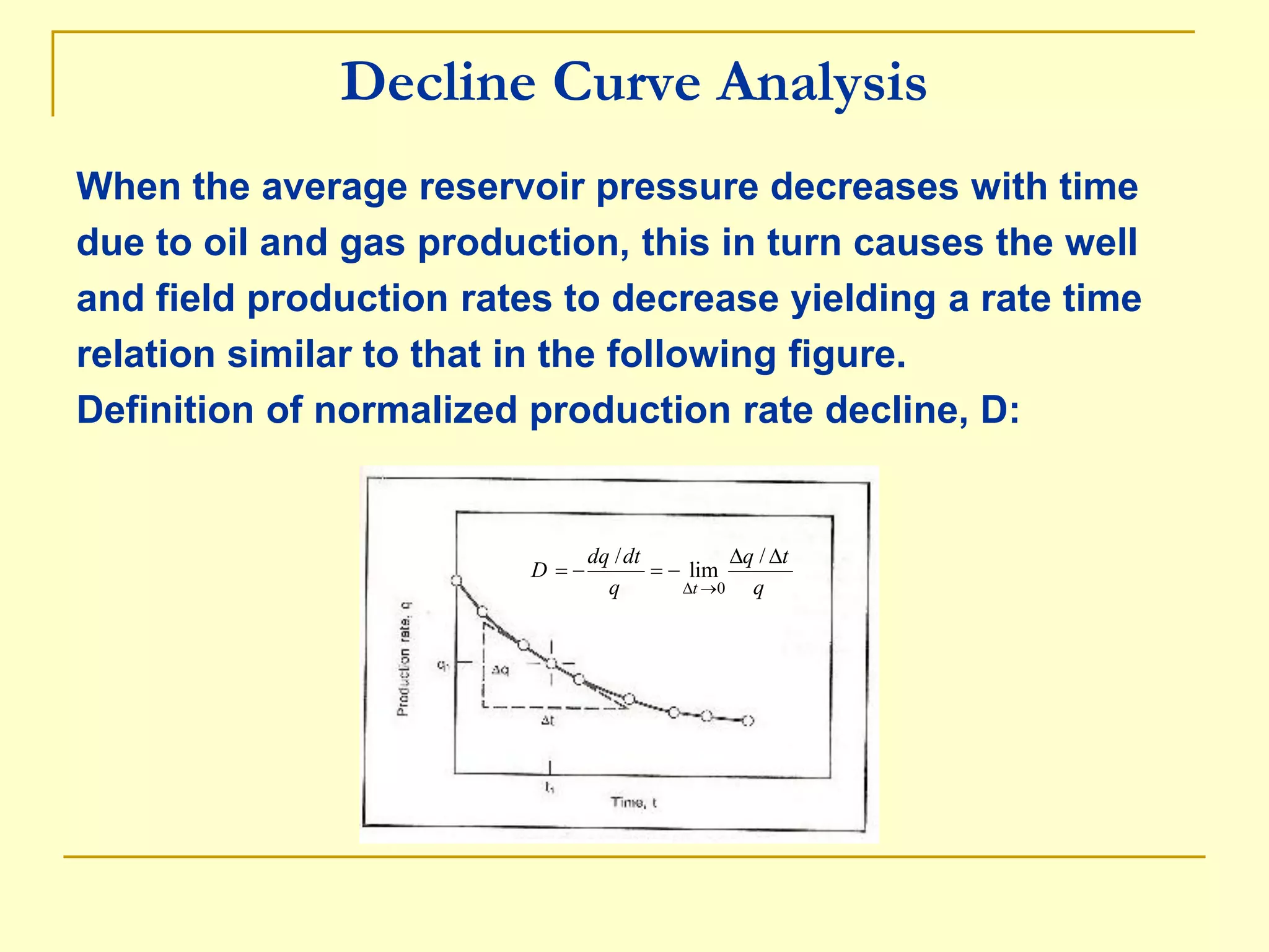
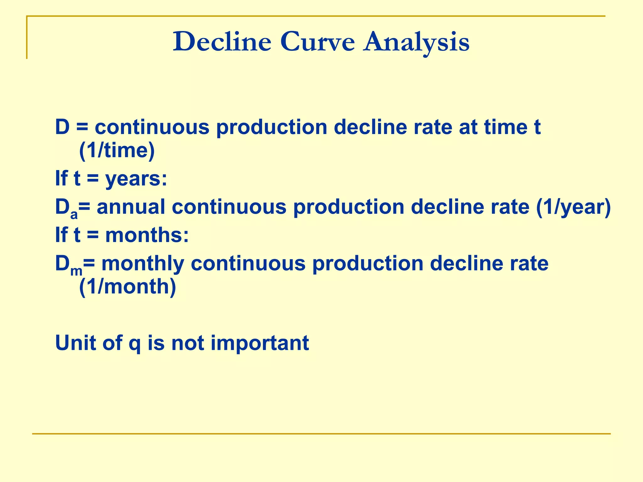
1. Decline curve analysis models the production rate decline over time for oil and gas reservoirs and can be used to estimate reserves.
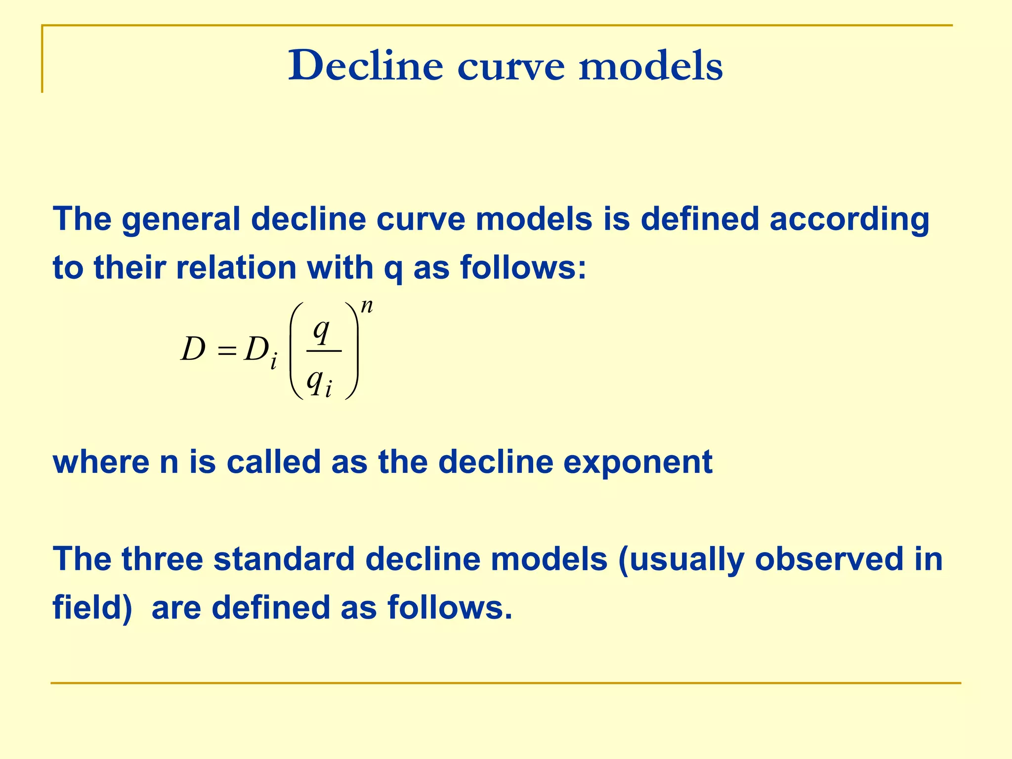
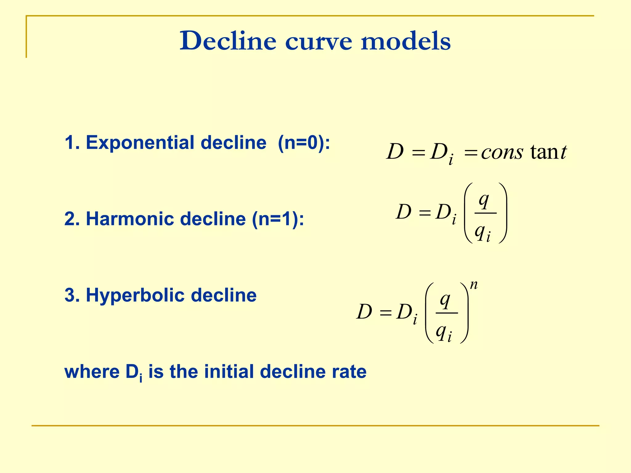
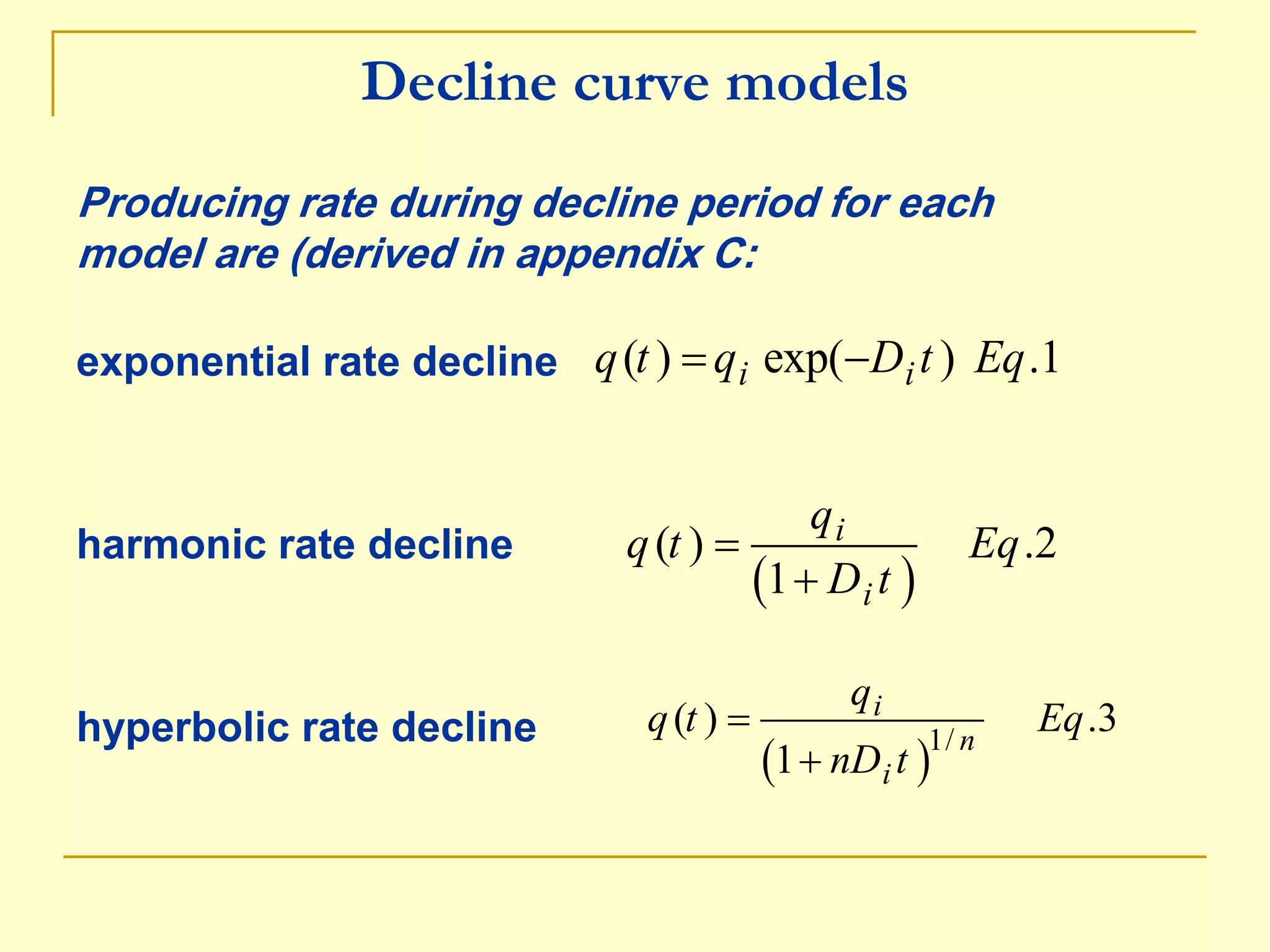
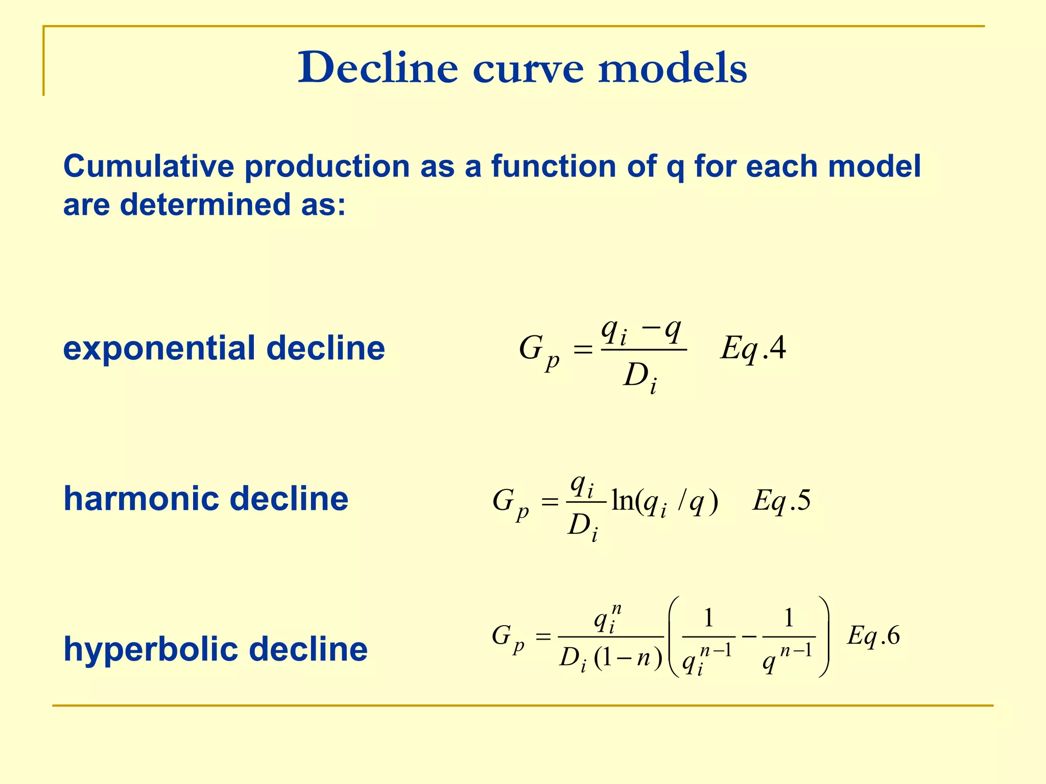
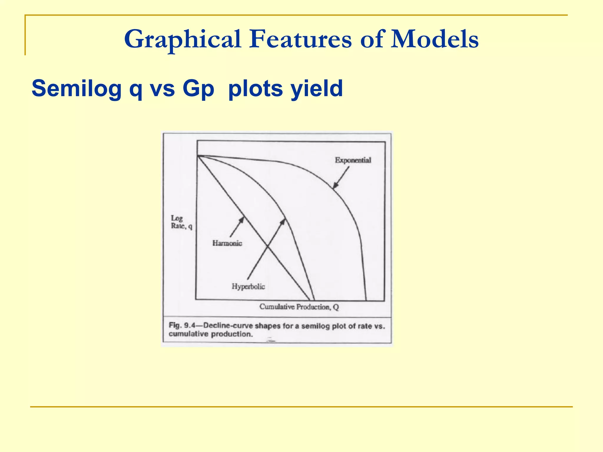
2. There are three standard decline curves that are commonly observed: exponential, harmonic, and hyperbolic decline. Different decline curves have different mathematical formulas to model the production rate decline.
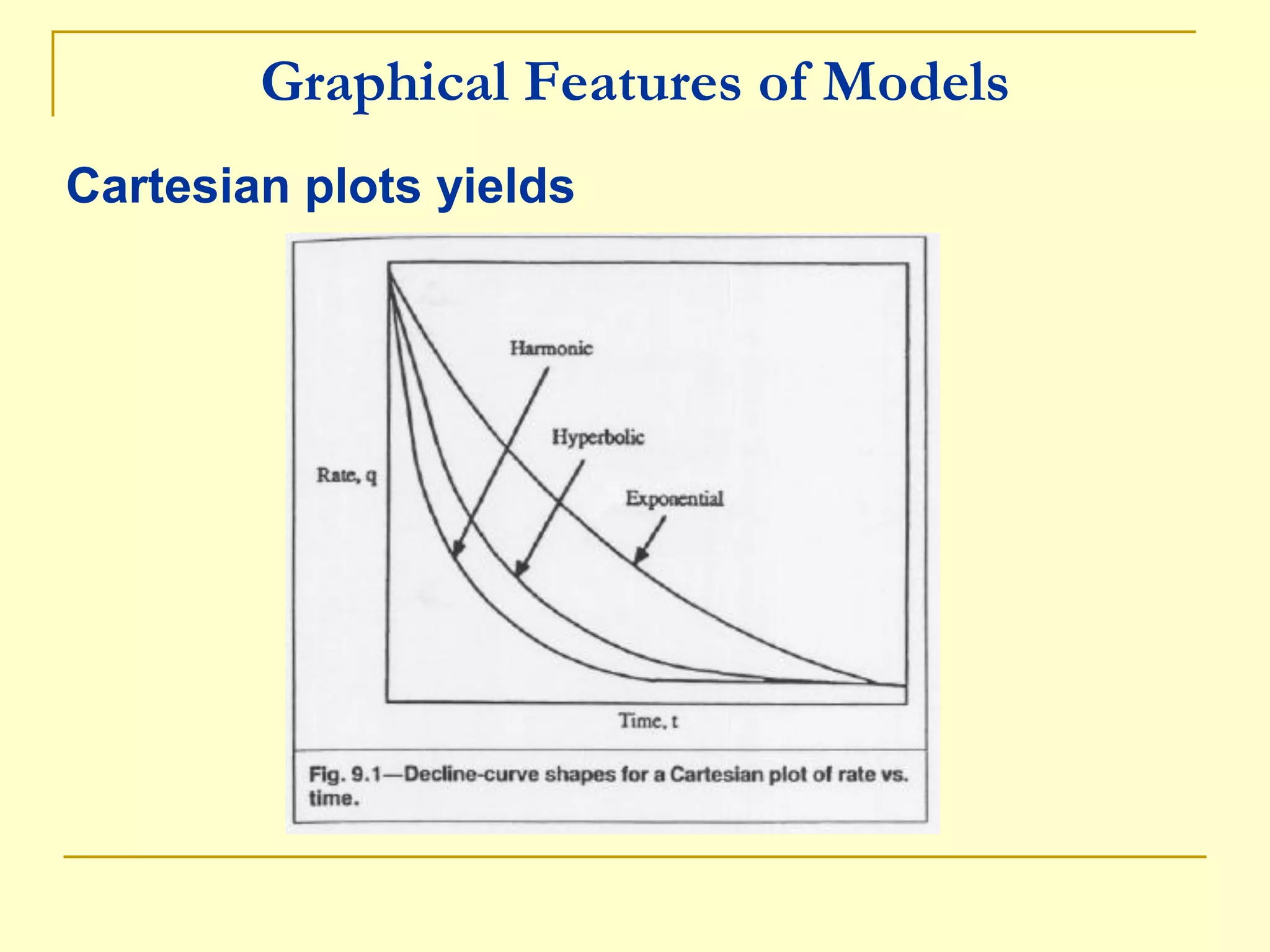
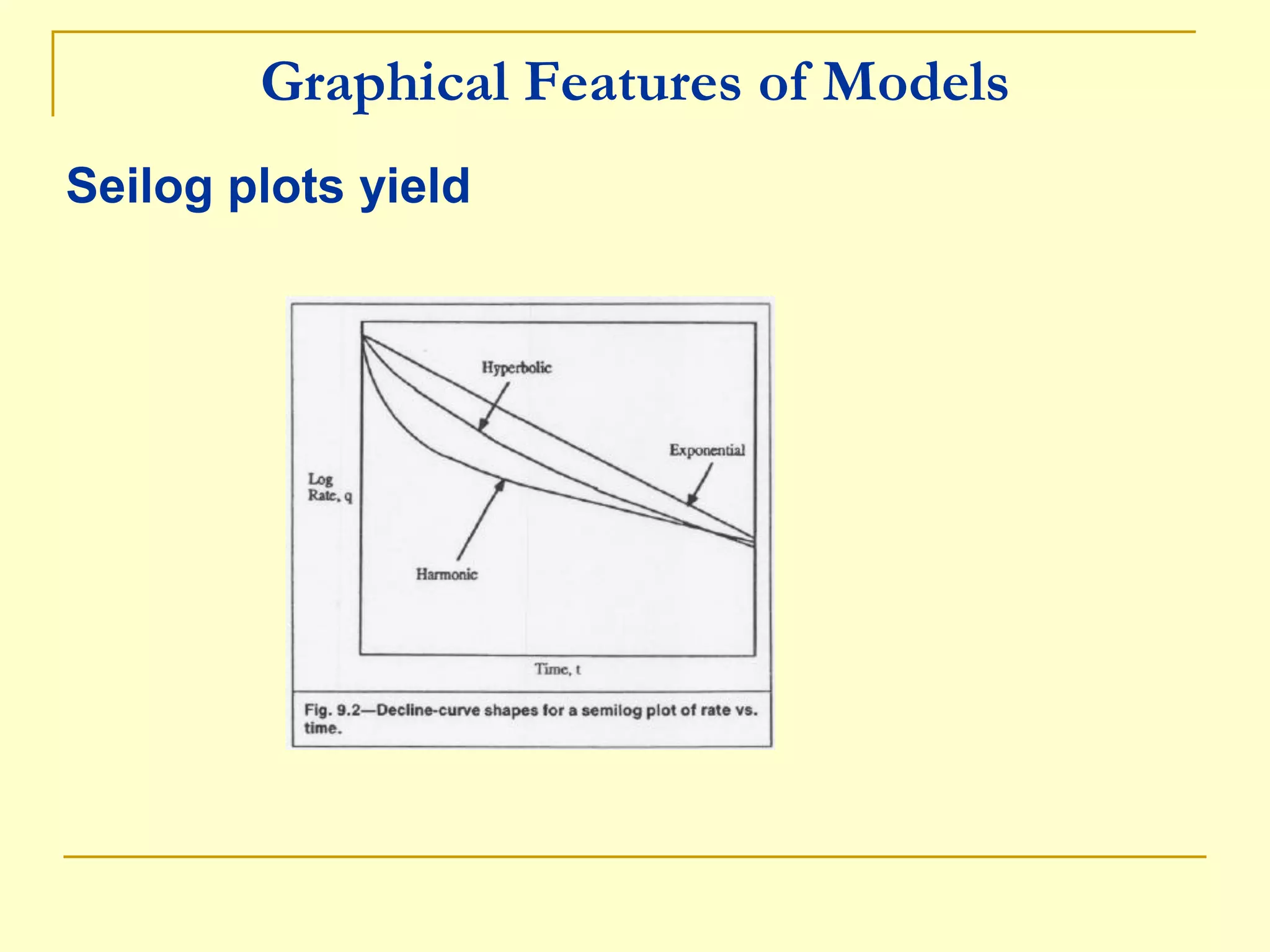
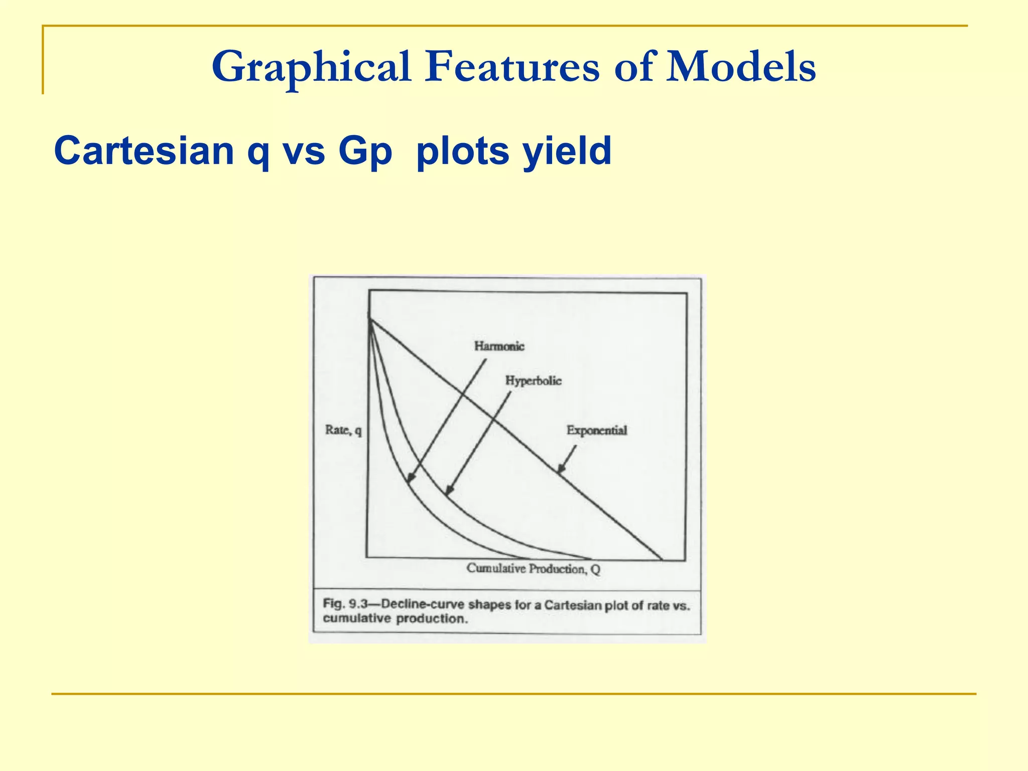
3. Production decline plots like log(rate) vs. time can identify the type of decline curve and be used to determine the curve parameters to forecast future production. Nonlinear regression is recommended for fitting hyperbolic decline curves.