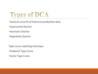
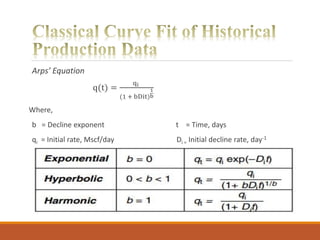
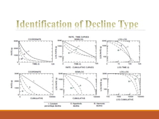
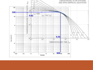
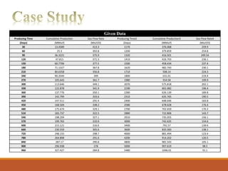
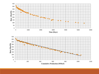
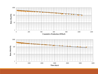
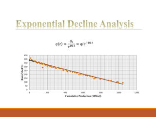
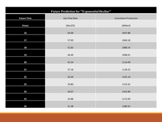
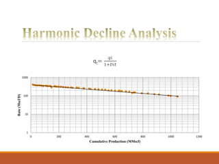
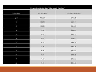
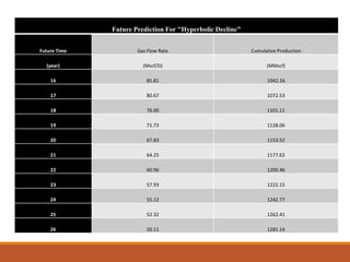
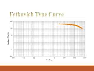
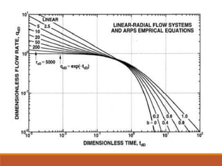
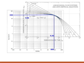
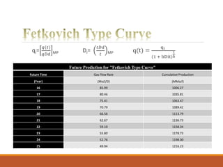
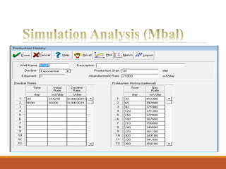
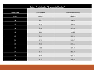
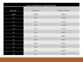
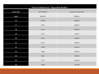
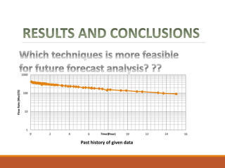
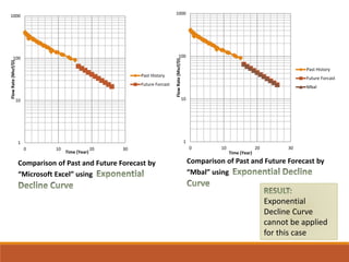
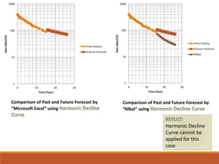
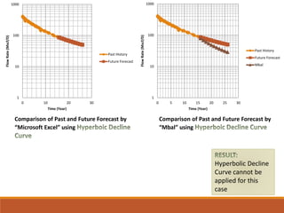
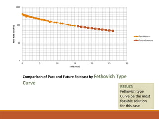
SlideShare a Scribd company logo
1 of 51
•Importance
•Unconventional reservoirs
•Arps Vs. Fetkovich type
•Requires less data and give better estimates
“Overview of proposed method to calculate reserves
for conventional reservoirs and interpretation of case
study using Microsoft Excel and MBAL”
Identification
of hyperbolic
decline family
equation using
graphical
analysis
Predict the
future forecast
using hyperbolic
family equation
aided by
Fetkovich type
curve
We compared the
actual production
data and the
generated data and
studied the impacts
on our results.
We find out
declining rate
using the
corresponding
the hyperbolic
family equation
In the second part a
base model was
considered using
commercial available
software to replicate
one of the case
history using
Fetkovich type
curve.
•Effective future forecast
•Overview of composite profile decline curve
analysis
•Comparative Analysis between MICROSOFT
EXCEL & MBAL
•Economic time limit computation more precisely
•More precise forecast analysis
•Effective computation of recoverable reserves
Introduction to DCA
Classical curve fit of historical production data
•Exponential Decline
•Harmonic Decline
•Hyperbolic Decline
Type-curve matching technique
•Fetkovich Type Curve
•Carter Type Curve
Arps’ Equation
q(t) =
qi
(1 + bDit)
1
b
Where,
b = Decline exponent t = Time, days
qi = Initial rate, Mscf/day Di = Initial decline rate, day-1
Decline curves characterized by 3 factors:
Initial Production Rate
Curvature of decline
Rate of decline
Ikuko Analysis
Production must Have been stable
Stable reservoir conditions
DCA is used in evaluation of new investment
•Stable production
•Stable reservoir conditions
•Boundary dominant conditions
Theoretical plots of solutions.
 Uses log-log graph.
Find the flow characteristics of individual well.
• Fetkovich Type Curve
•Carter Type Curve
Based on analytical solutions
Can be used for analyzing hydraulically fractured wells
Include both flow regimes.
Plot q(t) & Gp (t) vs time on log-log paper
Match the production data to the best fitting type curve
Record the values of corresponding parameters.
ASSUUMPTIONS:
•Constant BHP
•Permeability and skin
•Boundary Conditions
•Volumetric Reservoir
•Fetkovich (1980)
•Holditch (2006)
•Holditch and Madani (2010)
•Naik (2013)
Given Data
Producing Time Cumulative Production Gas Flow Rate Producing Time2 Cumulative Production3 Gas Flow Rate4
(Days) (MMscf) (Mscf/D) (Days) (MMscf) (Mscf/D)
30 13.4589 413.3 1170 376.068 259.9
60 25.3 392.8 1200 379.859 254.8
90 36.3221 375.9 1320 416.501 249.54
120 47.815 371.3 1410 426.793 236.1
150 60.7706 377.5 1500 458.434 237.4
180 71.1327 367.8 1620 482.743 230.1
210 80.6358 356.8 1710 508.14 224.3
240 90.3544 349 1800 531.01 219.4
270 105.643 361.7 1980 554.58 199.9
300 113.646 349.1 2070 575.818 202.1
330 122.878 341.9 2190 601.082 196.4
360 137.776 350.1 2280 626.139 189.8
390 142.799 333.6 2310 635.765 190.5
420 147.511 291.4 2400 648.646 183.8
450 168.504 338.2 2580 678.628 176.4
480 175.674 329.1 2700 702.659 170.3
510 183.737 322.5 2880 722.806 143.7
540 198.204 327.1 2910 735.055 156.1
570 199.765 310.9 3000 742.635 154.6
600 215.121 316.6 3400 791.57 139.6
660 230.559 305.6 3600 835.583 138.1
720 248.155 298.7 4000 881.494 123.4
780 264.898 291.6 4200 914.202 120.5
840 287.17 290.8 4800 981.543 105.1
900 296.938 278 5000 997.619 98.5
960 327.427 284.8 5480 1046.01 91.1
0
50
100
150
200
250
300
350
400
450
0 1000 2000 3000 4000 5000 6000
Rate(Mscf/D)
Time (Days)
0
50
100
150
200
250
300
350
400
450
0 200 400 600 800 1000 1200
Rate(Mscf/D)
Cumulative Production (MMscf)
1
10
100
1000
0 200 400 600 800 1000 1200
Rate(Mscf/D)
Cumulative Production (MMscf)
1
10
100
1000
0 1000 2000 3000 4000 5000 6000
Rate(MScf/D)
Time (days)
0
50
100
150
200
250
300
350
400
450
0 200 400 600 800 1000 1200
Rate(Mscf/D)
Cumulative Production (MMscf)
𝑞 𝑡 =
𝑞𝑖
𝑒 𝐷𝑖 𝑡
= 𝑞𝑖𝑒−𝐷𝑖 𝑡
Future Prediction for "Exponential Decline"
Future Time Gas Flow Rate Cumulative Production
(Year) (Mscf/D) (MMscf)
16 64.68 1037.88
17 57.90 1060.18
18 51.83 1080.14
19 46.40 1098.01
20 41.54 1114.00
21 37.18 1128.32
22 33.29 1141.14
23 29.80 1152.62
24 26.67 1162.89
25 23.88 1172.09
26 21.38 1180.32
qt=
𝑞i
1+𝐷𝑖𝑡
1
10
100
1000
0 200 400 600 800 1000 1200
Rate(Mscf/D)
Cumulative Production (MMscf)
Future Prediction For "Harmonic Decline"
Future Time Gas Flow Rate Cumulative Production
(year) (Mscf/D) (MMscf)
16 105.98 1126.44
17 101.29 1164.25
18 97.00 1200.43
19 93.07 1235.11
20 89.43 1268.41
21 86.07 1300.44
22 82.96 1331.28
23 80.06 1361.03
24 77.36 1389.75
25 74.83 1417.52
26 72.47 1444.40
qt =
𝑞𝑖
(1+𝐷𝑖𝑏𝑡)1/𝑏
Iteration Technique
Future Prediction For "Hyperbolic Decline"
Future Time Gas Flow Rate Cumulative Production
(year) (Mscf/D) (MMscf)
16 85.81 1042.16
17 80.67 1072.53
18 76.00 1101.11
19 71.73 1128.06
20 67.83 1153.52
21 64.25 1177.62
22 60.96 1200.46
23 57.93 1222.15
24 55.12 1242.77
25 52.32 1262.41
26 50.11 1281.14
0.01
0.1
1
10
100
1000
0.001 0.01 0.1 1 10 100 1000 10000
GasRate(Mscf/D)
Time (Days)
qi=
𝑞(𝑡)
𝑞𝐷𝑑 MP Di=
𝑡𝐷𝑑
𝑡 MP q(t) =
qi
(1 + bDit)
1
b
Future Prediction for "Fetkovich Type Curve"
Future Time Gas Flow Rate Cumulative Production
(Year) (Mscf/D) (MMscf)
16 85.99 1006.27
17 80.46 1035.81
18 75.41 1063.47
19 70.79 1089.42
20 66.56 1113.79
21 62.67 1136.73
22 59.10 1158.34
23 55.80 1178.73
24 52.76 1198.00
25 49.94 1216.23
Future Prediction for "Exponential Decline"
Future Time Gas Flow Rate Cumulative Production
(Year) (Mscf/D) (MMscf)
16 64.71 1030.95
17 57.91 1053.37
18 51.84 1073.38
19 46.42 1091.3
20 41.55 1107.34
21 37.18 1121.73
22 33.29 1134.58
23 29.8 1146.08
24 26.68 1156.38
25 23.88 1165.63
26 21.43 1173.71
Future Prediction For "Harmonic Decline“
Future Time Gas Flow Rate Cumulative Production
(year) (Mscf/D) (MMscf)
16 76.971 1076.06
17 66.61 1102.24
18 58.72 1125.06
19 52.51 1145.32
20 47.49 1163.54
21 43.33 1180.14
22 39.85 1195.3
23 36.89 1209.29
24 34.33 1222.28
25 32.11 1234.43
26 30.11 1245.55
Future Prediction For "Hyperbolic Decline"
Future Time Gas Flow Rate Cumulative Production
(year) (Mscf/D) (MMscf)
16 79.059 1058.03
17 69.31 1085.03
18 61.34 1108.92
19 54.72 1130.07
20 49.15 1148.99
21 44.41 1166.09
22 40.36 1181.55
23 36.86 1195.63
24 33.81 1208.51
25 31.11 1220.39
26 28.83 1231.08
1
10
100
1000
0 2 4 6 8 10 12 14 16
FlowRate(Mscf/D)
Time (Year)
Past history of given data
1
10
100
1000
0 10 20 30
FlowRate(Mscf/D)
Time (Year)
Past History
Future Forcast
1
10
100
1000
0 10 20 30
FlowRate(Mscf/D)
Time (Year)
Past History
Future Forcast
Mbal
Comparison of Past and Future Forecast by
“Microsoft Excel” using
Comparison of Past and Future Forecast by
“Mbal” using
Exponential
Decline Curve
cannot be applied
for this case
1
10
100
1000
0 10 20 30
Rate(Mscf/D)
Time (Year)
Past History
Future Forecast
1
10
100
1000
0 10 20 30
Rate(Mscf/D)
Time (Year)
Past History
Future Forecast
Mbal
Comparison of Past and Future Forecast by
“Microsoft Excel” using
Comparison of Past and Future Forecast by
“Mbal” using
Harmonic Decline
Curve cannot be
applied for this
case
1
10
100
1000
0 10 20 30
FlowRate(Mscf/D)
Time (Year)
Past History
Future Forecast
1
10
100
1000
0 5 10 15 20 25 30
FlowRate(Mscf/D)
Time (Year)
Past History
Future Forecast
Mbal
Comparison of Past and Future Forecast by
“Microsoft Excel” using
Hyperbolic Decline
Curve cannot be
applied for this
case
Comparison of Past and Future Forecast by
“Mbal” using
1
10
100
1000
0 5 10 15 20 25 30
FlowRate(Mscf/D)
Time (Year)
Past History
Future Forecast
Comparison of Past and Future Forecast by
Fetkovich type
Curve be the most
feasible solution
for this case
Excel Results
Exponential Harmonic Hyperbolic Type Curve
Time (Years) 22.92 70.77 40.01 35.42
G(P) (MMscf) 1153.87 2182.22 1348.12 1359.77
Recovery Factor(%) 92.26 43.4 61.55 62.67
Mbal Results
Column1 Exponential Harmonic Hyperbolic
Time (Years) 22.88 66.92 39.12
G(P) (MMscf) 1234.5 2049.74 1490.59
Recovery Factor(%) 99.21 43.19 67.32
Economic Limit q = 30 (Mscf/Day)
•DCA can be applied on any type of reservoir whether it is gas reservoir or oil reservoir
with equal accuracy & whether it is conventional one or unconventional and we just
need past production history.
•While applying DCA for unconventional reserves just keep in mind the very low
permeability factor because our reservoir should be in the pseudo steady state.
•DCA can be used to estimate ultimate gas recovery, remaining productive life of the
field at some abandonment pressure, drainage radius and pore volume, skin &
permeability of the reservoir.
•DCA is much more accurate and requires less data as compared to the
MBE technique and volumetric technique, since it predicts future
forecast using past production history and it accommodates the time
factor as well, i.e. how much time this reservoir will take to recover this
amount of reserves and in petroleum sector “time is money”.
•DCA can be applied only if the past production trends follows one of the “Hyperbolic
family of equations i.e. exponential, hyperbolic or harmonic trends”, if it is not
happening, we cannot estimate reserves in an effective way.
•DCA can only give precise future estimates if production controlling factors will
continue in the future following the past trends & production mechanism will remains
same e.g. if we install artificial lift system on a reservoir after DCA estimation, in that
case DCA results becomes erroneous.
•Utilize all available techniques:
Utilizes curve matching technique as well other than hyperbolic equations for
high effective results.
•Comparison between the data base and software base:
Use of data base and compares their results with commercial available
software to estimates better reserves.
•Utilize modern techniques for unconventional reservoirs:
Use of modern techniques like “Exponental+Hyperbolic decline” & “Power
exponential decline” for unconventional reservoirs etc.
https://www.onepetro.org/download/conference-paper/IPTC-18188-
MS?id=conference-paper%2FIPTC-18188-MS
https://www.onepetro.org/search?q=iptc-14801-
ms&peer_reviewed=&published_between=&from_year=&to_year=&rows=10
https://www.onepetro.org/download/conference-paper/SPE-170945-
MS?id=conference-paper%2FSPE-170945-MS
Reservoir Engineering Handbook by Tarek Ahmed (Fourth Edition)
John Lee and Robert A. Wattenbarger. Copyright 1996. Gas Reservoir
Engineering. Society of Petroleum Engineers Inc
E.I. Shirman. Universal Approach to Decline Curve Analysis. Louisiana State
University.
J.J Arps. 1994. Decline Curve Analysis. A.I.M.E
QESTIONS ARE
WELCOME…

More Related Content

What's hot

Q913 re1 w5 lec 18
Q913 re1 w5 lec 18Q913 re1 w5 lec 18
Q913 re1 w5 lec 18AFATous
 
Nodal Analysis introduction to inflow and outflow performance - next
Nodal Analysis   introduction to inflow and outflow performance - nextNodal Analysis   introduction to inflow and outflow performance - next
Nodal Analysis introduction to inflow and outflow performance - nextgusgon
 
Nsulangi_Drives Mechanism_CUG
Nsulangi_Drives Mechanism_CUGNsulangi_Drives Mechanism_CUG
Nsulangi_Drives Mechanism_CUGNsulangi Paul
 
reservoir engineering
reservoir engineeringreservoir engineering
reservoir engineeringbehnamproeng
 
Reservoir simulation (april 2017)
Reservoir simulation (april 2017)Reservoir simulation (april 2017)
Reservoir simulation (april 2017)NghiaHuynh47
 
Factors effecting vertical lift performance
Factors effecting vertical lift performanceFactors effecting vertical lift performance
Factors effecting vertical lift performanceJALEEL AHMED
 
Q913 re1 w4 lec 13
Q913 re1 w4 lec 13Q913 re1 w4 lec 13
Q913 re1 w4 lec 13AFATous
 
13 artificial-lift
13 artificial-lift13 artificial-lift
13 artificial-liftjuanca0106
 
Semester Project in Reservoir Simulation
Semester Project in Reservoir SimulationSemester Project in Reservoir Simulation
Semester Project in Reservoir SimulationKonstantinos D Pandis
 
Crude oil Production System
Crude oil Production System Crude oil Production System
Crude oil Production System Tobiloba Omitola
 
Rock Compressibility
Rock CompressibilityRock Compressibility
Rock CompressibilityM.T.H Group
 
CO2 EOR Pilot Project
CO2 EOR Pilot ProjectCO2 EOR Pilot Project
CO2 EOR Pilot ProjectAhmed Nour
 

What's hot (20)

Does Heavy Oil Recovery Need Steam?
Does Heavy Oil Recovery Need Steam?Does Heavy Oil Recovery Need Steam?
Does Heavy Oil Recovery Need Steam?
 
Field Development Plan
Field Development PlanField Development Plan
Field Development Plan
 
Well test analysis
Well test analysisWell test analysis
Well test analysis
 
Q913 re1 w5 lec 18
Q913 re1 w5 lec 18Q913 re1 w5 lec 18
Q913 re1 w5 lec 18
 
Reservoir
ReservoirReservoir
Reservoir
 
Nodal Analysis introduction to inflow and outflow performance - next
Nodal Analysis   introduction to inflow and outflow performance - nextNodal Analysis   introduction to inflow and outflow performance - next
Nodal Analysis introduction to inflow and outflow performance - next
 
Nsulangi_Drives Mechanism_CUG
Nsulangi_Drives Mechanism_CUGNsulangi_Drives Mechanism_CUG
Nsulangi_Drives Mechanism_CUG
 
reservoir engineering
reservoir engineeringreservoir engineering
reservoir engineering
 
Reservoir simulation (april 2017)
Reservoir simulation (april 2017)Reservoir simulation (april 2017)
Reservoir simulation (april 2017)
 
Factors effecting vertical lift performance
Factors effecting vertical lift performanceFactors effecting vertical lift performance
Factors effecting vertical lift performance
 
Q913 re1 w4 lec 13
Q913 re1 w4 lec 13Q913 re1 w4 lec 13
Q913 re1 w4 lec 13
 
Artificial Lift Methods
Artificial Lift MethodsArtificial Lift Methods
Artificial Lift Methods
 
Waterflood Design and Operational Best Practices
Waterflood Design and Operational Best PracticesWaterflood Design and Operational Best Practices
Waterflood Design and Operational Best Practices
 
Reservoir modeling and characterization
Reservoir modeling and characterizationReservoir modeling and characterization
Reservoir modeling and characterization
 
13 artificial-lift
13 artificial-lift13 artificial-lift
13 artificial-lift
 
Semester Project in Reservoir Simulation
Semester Project in Reservoir SimulationSemester Project in Reservoir Simulation
Semester Project in Reservoir Simulation
 
Water influx
Water influxWater influx
Water influx
 
Crude oil Production System
Crude oil Production System Crude oil Production System
Crude oil Production System
 
Rock Compressibility
Rock CompressibilityRock Compressibility
Rock Compressibility
 
CO2 EOR Pilot Project
CO2 EOR Pilot ProjectCO2 EOR Pilot Project
CO2 EOR Pilot Project
 

Similar to Presentation

Wavelet bootstrap Multiple linear regression models
Wavelet bootstrap Multiple linear regression modelsWavelet bootstrap Multiple linear regression models
Wavelet bootstrap Multiple linear regression modelsVinit Sehgal
 
University of Victoria Talk - Metocean analysis and Machine Learning for Impr...
University of Victoria Talk - Metocean analysis and Machine Learning for Impr...University of Victoria Talk - Metocean analysis and Machine Learning for Impr...
University of Victoria Talk - Metocean analysis and Machine Learning for Impr...Aaron Barker
 
IPPTChap010.pptx
IPPTChap010.pptxIPPTChap010.pptx
IPPTChap010.pptxQuangLong44
 
Flight Delay Prediction Model (2)
Flight Delay Prediction Model (2)Flight Delay Prediction Model (2)
Flight Delay Prediction Model (2)Shubham Gupta
 
Proposal Wide Blower No.1 & 2 with inverter
Proposal Wide Blower No.1 & 2  with inverterProposal Wide Blower No.1 & 2  with inverter
Proposal Wide Blower No.1 & 2 with inverterRidhoIrawan12
 
Peak shaving of an EV Aggregator Using Quadratic Programming
Peak shaving of an EV Aggregator Using Quadratic ProgrammingPeak shaving of an EV Aggregator Using Quadratic Programming
Peak shaving of an EV Aggregator Using Quadratic ProgrammingDaisuke Kodaira
 
Traffic state estimation with multi-sensor data for large networks with macro...
Traffic state estimation with multi-sensor data for large networks with macro...Traffic state estimation with multi-sensor data for large networks with macro...
Traffic state estimation with multi-sensor data for large networks with macro...YazanSafadi
 
Statistical quality control
Statistical quality controlStatistical quality control
Statistical quality controlSai Datri Arige
 
Mtc oil and gas use cases 05 16-2018
Mtc oil and gas use cases 05 16-2018Mtc oil and gas use cases 05 16-2018
Mtc oil and gas use cases 05 16-2018Dania Kodeih
 
Safran Colibrys MS1010 and MEMSIC MXA2500M High-End Accelerometers
Safran Colibrys MS1010 and MEMSIC MXA2500M High-End AccelerometersSafran Colibrys MS1010 and MEMSIC MXA2500M High-End Accelerometers
Safran Colibrys MS1010 and MEMSIC MXA2500M High-End Accelerometerssystem_plus
 
2018 National Tanks Conference & Exposition: HRSC Data Visualization
2018 National Tanks Conference & Exposition: HRSC Data Visualization2018 National Tanks Conference & Exposition: HRSC Data Visualization
2018 National Tanks Conference & Exposition: HRSC Data VisualizationAntea Group
 
Unconventional Data-Driven Methodologies Forecast Performance
Unconventional Data-Driven Methodologies Forecast PerformanceUnconventional Data-Driven Methodologies Forecast Performance
Unconventional Data-Driven Methodologies Forecast PerformanceKaanthan Shanmugam
 
Statistical Forecasting of Lightning Cessation _ PPT Presentation
Statistical Forecasting of Lightning Cessation _ PPT PresentationStatistical Forecasting of Lightning Cessation _ PPT Presentation
Statistical Forecasting of Lightning Cessation _ PPT PresentationJames Ervin Glover, Ph.D.
 
Waterfall Turbine Development Primer - Updated
Waterfall Turbine Development Primer - UpdatedWaterfall Turbine Development Primer - Updated
Waterfall Turbine Development Primer - UpdatedJason Rota
 
Wet x dry completion with risk
Wet x dry completion with riskWet x dry completion with risk
Wet x dry completion with riskGláucio Bastos
 
How Idaho Power Company uses AURORAxmp
How Idaho Power Company uses AURORAxmpHow Idaho Power Company uses AURORAxmp
How Idaho Power Company uses AURORAxmpEPIS Inc
 
Backscatter Working Group Software Inter-comparison Project Requesting and Co...
Backscatter Working Group Software Inter-comparison ProjectRequesting and Co...Backscatter Working Group Software Inter-comparison ProjectRequesting and Co...
Backscatter Working Group Software Inter-comparison Project Requesting and Co...Giuseppe Masetti
 
الدكتور / علي المراكبي استشاري الهندسة الميكانيكية وخبير ترشيد الطاقة بعنوان...
 الدكتور / علي المراكبي استشاري الهندسة الميكانيكية وخبير ترشيد الطاقة بعنوان... الدكتور / علي المراكبي استشاري الهندسة الميكانيكية وخبير ترشيد الطاقة بعنوان...
الدكتور / علي المراكبي استشاري الهندسة الميكانيكية وخبير ترشيد الطاقة بعنوان...Egyptian Engineers Association
 

Similar to Presentation (20)

Wavelet bootstrap Multiple linear regression models
Wavelet bootstrap Multiple linear regression modelsWavelet bootstrap Multiple linear regression models
Wavelet bootstrap Multiple linear regression models
 
Forecasting Assignment Help
Forecasting Assignment HelpForecasting Assignment Help
Forecasting Assignment Help
 
University of Victoria Talk - Metocean analysis and Machine Learning for Impr...
University of Victoria Talk - Metocean analysis and Machine Learning for Impr...University of Victoria Talk - Metocean analysis and Machine Learning for Impr...
University of Victoria Talk - Metocean analysis and Machine Learning for Impr...
 
IPPTChap010.pptx
IPPTChap010.pptxIPPTChap010.pptx
IPPTChap010.pptx
 
Flight Delay Prediction Model (2)
Flight Delay Prediction Model (2)Flight Delay Prediction Model (2)
Flight Delay Prediction Model (2)
 
Proposal Wide Blower No.1 & 2 with inverter
Proposal Wide Blower No.1 & 2  with inverterProposal Wide Blower No.1 & 2  with inverter
Proposal Wide Blower No.1 & 2 with inverter
 
Peak shaving of an EV Aggregator Using Quadratic Programming
Peak shaving of an EV Aggregator Using Quadratic ProgrammingPeak shaving of an EV Aggregator Using Quadratic Programming
Peak shaving of an EV Aggregator Using Quadratic Programming
 
Travel_Time_Reliability
Travel_Time_ReliabilityTravel_Time_Reliability
Travel_Time_Reliability
 
Traffic state estimation with multi-sensor data for large networks with macro...
Traffic state estimation with multi-sensor data for large networks with macro...Traffic state estimation with multi-sensor data for large networks with macro...
Traffic state estimation with multi-sensor data for large networks with macro...
 
Statistical quality control
Statistical quality controlStatistical quality control
Statistical quality control
 
Mtc oil and gas use cases 05 16-2018
Mtc oil and gas use cases 05 16-2018Mtc oil and gas use cases 05 16-2018
Mtc oil and gas use cases 05 16-2018
 
Safran Colibrys MS1010 and MEMSIC MXA2500M High-End Accelerometers
Safran Colibrys MS1010 and MEMSIC MXA2500M High-End AccelerometersSafran Colibrys MS1010 and MEMSIC MXA2500M High-End Accelerometers
Safran Colibrys MS1010 and MEMSIC MXA2500M High-End Accelerometers
 
2018 National Tanks Conference & Exposition: HRSC Data Visualization
2018 National Tanks Conference & Exposition: HRSC Data Visualization2018 National Tanks Conference & Exposition: HRSC Data Visualization
2018 National Tanks Conference & Exposition: HRSC Data Visualization
 
Unconventional Data-Driven Methodologies Forecast Performance
Unconventional Data-Driven Methodologies Forecast PerformanceUnconventional Data-Driven Methodologies Forecast Performance
Unconventional Data-Driven Methodologies Forecast Performance
 
Statistical Forecasting of Lightning Cessation _ PPT Presentation
Statistical Forecasting of Lightning Cessation _ PPT PresentationStatistical Forecasting of Lightning Cessation _ PPT Presentation
Statistical Forecasting of Lightning Cessation _ PPT Presentation
 
Waterfall Turbine Development Primer - Updated
Waterfall Turbine Development Primer - UpdatedWaterfall Turbine Development Primer - Updated
Waterfall Turbine Development Primer - Updated
 
Wet x dry completion with risk
Wet x dry completion with riskWet x dry completion with risk
Wet x dry completion with risk
 
How Idaho Power Company uses AURORAxmp
How Idaho Power Company uses AURORAxmpHow Idaho Power Company uses AURORAxmp
How Idaho Power Company uses AURORAxmp
 
Backscatter Working Group Software Inter-comparison Project Requesting and Co...
Backscatter Working Group Software Inter-comparison ProjectRequesting and Co...Backscatter Working Group Software Inter-comparison ProjectRequesting and Co...
Backscatter Working Group Software Inter-comparison Project Requesting and Co...
 
الدكتور / علي المراكبي استشاري الهندسة الميكانيكية وخبير ترشيد الطاقة بعنوان...
 الدكتور / علي المراكبي استشاري الهندسة الميكانيكية وخبير ترشيد الطاقة بعنوان... الدكتور / علي المراكبي استشاري الهندسة الميكانيكية وخبير ترشيد الطاقة بعنوان...
الدكتور / علي المراكبي استشاري الهندسة الميكانيكية وخبير ترشيد الطاقة بعنوان...
 

Presentation

  • 1.
  • 2.
  • 3.
  • 4.
  • 5. •Importance •Unconventional reservoirs •Arps Vs. Fetkovich type •Requires less data and give better estimates
  • 6. “Overview of proposed method to calculate reserves for conventional reservoirs and interpretation of case study using Microsoft Excel and MBAL”
  • 7. Identification of hyperbolic decline family equation using graphical analysis Predict the future forecast using hyperbolic family equation aided by Fetkovich type curve We compared the actual production data and the generated data and studied the impacts on our results. We find out declining rate using the corresponding the hyperbolic family equation In the second part a base model was considered using commercial available software to replicate one of the case history using Fetkovich type curve.
  • 8. •Effective future forecast •Overview of composite profile decline curve analysis •Comparative Analysis between MICROSOFT EXCEL & MBAL
  • 9. •Economic time limit computation more precisely •More precise forecast analysis •Effective computation of recoverable reserves
  • 11. Classical curve fit of historical production data •Exponential Decline •Harmonic Decline •Hyperbolic Decline Type-curve matching technique •Fetkovich Type Curve •Carter Type Curve
  • 12. Arps’ Equation q(t) = qi (1 + bDit) 1 b Where, b = Decline exponent t = Time, days qi = Initial rate, Mscf/day Di = Initial decline rate, day-1
  • 13.
  • 14. Decline curves characterized by 3 factors: Initial Production Rate Curvature of decline Rate of decline Ikuko Analysis Production must Have been stable Stable reservoir conditions DCA is used in evaluation of new investment
  • 15. •Stable production •Stable reservoir conditions •Boundary dominant conditions
  • 16. Theoretical plots of solutions.  Uses log-log graph. Find the flow characteristics of individual well.
  • 17. • Fetkovich Type Curve •Carter Type Curve
  • 18. Based on analytical solutions Can be used for analyzing hydraulically fractured wells Include both flow regimes.
  • 19. Plot q(t) & Gp (t) vs time on log-log paper Match the production data to the best fitting type curve Record the values of corresponding parameters.
  • 20.
  • 21. ASSUUMPTIONS: •Constant BHP •Permeability and skin •Boundary Conditions •Volumetric Reservoir
  • 22. •Fetkovich (1980) •Holditch (2006) •Holditch and Madani (2010) •Naik (2013)
  • 23. Given Data Producing Time Cumulative Production Gas Flow Rate Producing Time2 Cumulative Production3 Gas Flow Rate4 (Days) (MMscf) (Mscf/D) (Days) (MMscf) (Mscf/D) 30 13.4589 413.3 1170 376.068 259.9 60 25.3 392.8 1200 379.859 254.8 90 36.3221 375.9 1320 416.501 249.54 120 47.815 371.3 1410 426.793 236.1 150 60.7706 377.5 1500 458.434 237.4 180 71.1327 367.8 1620 482.743 230.1 210 80.6358 356.8 1710 508.14 224.3 240 90.3544 349 1800 531.01 219.4 270 105.643 361.7 1980 554.58 199.9 300 113.646 349.1 2070 575.818 202.1 330 122.878 341.9 2190 601.082 196.4 360 137.776 350.1 2280 626.139 189.8 390 142.799 333.6 2310 635.765 190.5 420 147.511 291.4 2400 648.646 183.8 450 168.504 338.2 2580 678.628 176.4 480 175.674 329.1 2700 702.659 170.3 510 183.737 322.5 2880 722.806 143.7 540 198.204 327.1 2910 735.055 156.1 570 199.765 310.9 3000 742.635 154.6 600 215.121 316.6 3400 791.57 139.6 660 230.559 305.6 3600 835.583 138.1 720 248.155 298.7 4000 881.494 123.4 780 264.898 291.6 4200 914.202 120.5 840 287.17 290.8 4800 981.543 105.1 900 296.938 278 5000 997.619 98.5 960 327.427 284.8 5480 1046.01 91.1
  • 24. 0 50 100 150 200 250 300 350 400 450 0 1000 2000 3000 4000 5000 6000 Rate(Mscf/D) Time (Days) 0 50 100 150 200 250 300 350 400 450 0 200 400 600 800 1000 1200 Rate(Mscf/D) Cumulative Production (MMscf)
  • 25. 1 10 100 1000 0 200 400 600 800 1000 1200 Rate(Mscf/D) Cumulative Production (MMscf) 1 10 100 1000 0 1000 2000 3000 4000 5000 6000 Rate(MScf/D) Time (days)
  • 26. 0 50 100 150 200 250 300 350 400 450 0 200 400 600 800 1000 1200 Rate(Mscf/D) Cumulative Production (MMscf) 𝑞 𝑡 = 𝑞𝑖 𝑒 𝐷𝑖 𝑡 = 𝑞𝑖𝑒−𝐷𝑖 𝑡
  • 27. Future Prediction for "Exponential Decline" Future Time Gas Flow Rate Cumulative Production (Year) (Mscf/D) (MMscf) 16 64.68 1037.88 17 57.90 1060.18 18 51.83 1080.14 19 46.40 1098.01 20 41.54 1114.00 21 37.18 1128.32 22 33.29 1141.14 23 29.80 1152.62 24 26.67 1162.89 25 23.88 1172.09 26 21.38 1180.32
  • 28. qt= 𝑞i 1+𝐷𝑖𝑡 1 10 100 1000 0 200 400 600 800 1000 1200 Rate(Mscf/D) Cumulative Production (MMscf)
  • 29. Future Prediction For "Harmonic Decline" Future Time Gas Flow Rate Cumulative Production (year) (Mscf/D) (MMscf) 16 105.98 1126.44 17 101.29 1164.25 18 97.00 1200.43 19 93.07 1235.11 20 89.43 1268.41 21 86.07 1300.44 22 82.96 1331.28 23 80.06 1361.03 24 77.36 1389.75 25 74.83 1417.52 26 72.47 1444.40
  • 31. Future Prediction For "Hyperbolic Decline" Future Time Gas Flow Rate Cumulative Production (year) (Mscf/D) (MMscf) 16 85.81 1042.16 17 80.67 1072.53 18 76.00 1101.11 19 71.73 1128.06 20 67.83 1153.52 21 64.25 1177.62 22 60.96 1200.46 23 57.93 1222.15 24 55.12 1242.77 25 52.32 1262.41 26 50.11 1281.14
  • 32. 0.01 0.1 1 10 100 1000 0.001 0.01 0.1 1 10 100 1000 10000 GasRate(Mscf/D) Time (Days)
  • 33.
  • 34.
  • 35. qi= 𝑞(𝑡) 𝑞𝐷𝑑 MP Di= 𝑡𝐷𝑑 𝑡 MP q(t) = qi (1 + bDit) 1 b Future Prediction for "Fetkovich Type Curve" Future Time Gas Flow Rate Cumulative Production (Year) (Mscf/D) (MMscf) 16 85.99 1006.27 17 80.46 1035.81 18 75.41 1063.47 19 70.79 1089.42 20 66.56 1113.79 21 62.67 1136.73 22 59.10 1158.34 23 55.80 1178.73 24 52.76 1198.00 25 49.94 1216.23
  • 36.
  • 37. Future Prediction for "Exponential Decline" Future Time Gas Flow Rate Cumulative Production (Year) (Mscf/D) (MMscf) 16 64.71 1030.95 17 57.91 1053.37 18 51.84 1073.38 19 46.42 1091.3 20 41.55 1107.34 21 37.18 1121.73 22 33.29 1134.58 23 29.8 1146.08 24 26.68 1156.38 25 23.88 1165.63 26 21.43 1173.71
  • 38. Future Prediction For "Harmonic Decline“ Future Time Gas Flow Rate Cumulative Production (year) (Mscf/D) (MMscf) 16 76.971 1076.06 17 66.61 1102.24 18 58.72 1125.06 19 52.51 1145.32 20 47.49 1163.54 21 43.33 1180.14 22 39.85 1195.3 23 36.89 1209.29 24 34.33 1222.28 25 32.11 1234.43 26 30.11 1245.55
  • 39. Future Prediction For "Hyperbolic Decline" Future Time Gas Flow Rate Cumulative Production (year) (Mscf/D) (MMscf) 16 79.059 1058.03 17 69.31 1085.03 18 61.34 1108.92 19 54.72 1130.07 20 49.15 1148.99 21 44.41 1166.09 22 40.36 1181.55 23 36.86 1195.63 24 33.81 1208.51 25 31.11 1220.39 26 28.83 1231.08
  • 40. 1 10 100 1000 0 2 4 6 8 10 12 14 16 FlowRate(Mscf/D) Time (Year) Past history of given data
  • 41. 1 10 100 1000 0 10 20 30 FlowRate(Mscf/D) Time (Year) Past History Future Forcast 1 10 100 1000 0 10 20 30 FlowRate(Mscf/D) Time (Year) Past History Future Forcast Mbal Comparison of Past and Future Forecast by “Microsoft Excel” using Comparison of Past and Future Forecast by “Mbal” using Exponential Decline Curve cannot be applied for this case
  • 42. 1 10 100 1000 0 10 20 30 Rate(Mscf/D) Time (Year) Past History Future Forecast 1 10 100 1000 0 10 20 30 Rate(Mscf/D) Time (Year) Past History Future Forecast Mbal Comparison of Past and Future Forecast by “Microsoft Excel” using Comparison of Past and Future Forecast by “Mbal” using Harmonic Decline Curve cannot be applied for this case
  • 43. 1 10 100 1000 0 10 20 30 FlowRate(Mscf/D) Time (Year) Past History Future Forecast 1 10 100 1000 0 5 10 15 20 25 30 FlowRate(Mscf/D) Time (Year) Past History Future Forecast Mbal Comparison of Past and Future Forecast by “Microsoft Excel” using Hyperbolic Decline Curve cannot be applied for this case Comparison of Past and Future Forecast by “Mbal” using
  • 44. 1 10 100 1000 0 5 10 15 20 25 30 FlowRate(Mscf/D) Time (Year) Past History Future Forecast Comparison of Past and Future Forecast by Fetkovich type Curve be the most feasible solution for this case
  • 45. Excel Results Exponential Harmonic Hyperbolic Type Curve Time (Years) 22.92 70.77 40.01 35.42 G(P) (MMscf) 1153.87 2182.22 1348.12 1359.77 Recovery Factor(%) 92.26 43.4 61.55 62.67 Mbal Results Column1 Exponential Harmonic Hyperbolic Time (Years) 22.88 66.92 39.12 G(P) (MMscf) 1234.5 2049.74 1490.59 Recovery Factor(%) 99.21 43.19 67.32 Economic Limit q = 30 (Mscf/Day)
  • 46. •DCA can be applied on any type of reservoir whether it is gas reservoir or oil reservoir with equal accuracy & whether it is conventional one or unconventional and we just need past production history. •While applying DCA for unconventional reserves just keep in mind the very low permeability factor because our reservoir should be in the pseudo steady state. •DCA can be used to estimate ultimate gas recovery, remaining productive life of the field at some abandonment pressure, drainage radius and pore volume, skin & permeability of the reservoir.
  • 47. •DCA is much more accurate and requires less data as compared to the MBE technique and volumetric technique, since it predicts future forecast using past production history and it accommodates the time factor as well, i.e. how much time this reservoir will take to recover this amount of reserves and in petroleum sector “time is money”.
  • 48. •DCA can be applied only if the past production trends follows one of the “Hyperbolic family of equations i.e. exponential, hyperbolic or harmonic trends”, if it is not happening, we cannot estimate reserves in an effective way. •DCA can only give precise future estimates if production controlling factors will continue in the future following the past trends & production mechanism will remains same e.g. if we install artificial lift system on a reservoir after DCA estimation, in that case DCA results becomes erroneous.
  • 49. •Utilize all available techniques: Utilizes curve matching technique as well other than hyperbolic equations for high effective results. •Comparison between the data base and software base: Use of data base and compares their results with commercial available software to estimates better reserves. •Utilize modern techniques for unconventional reservoirs: Use of modern techniques like “Exponental+Hyperbolic decline” & “Power exponential decline” for unconventional reservoirs etc.
  • 50. https://www.onepetro.org/download/conference-paper/IPTC-18188- MS?id=conference-paper%2FIPTC-18188-MS https://www.onepetro.org/search?q=iptc-14801- ms&peer_reviewed=&published_between=&from_year=&to_year=&rows=10 https://www.onepetro.org/download/conference-paper/SPE-170945- MS?id=conference-paper%2FSPE-170945-MS Reservoir Engineering Handbook by Tarek Ahmed (Fourth Edition) John Lee and Robert A. Wattenbarger. Copyright 1996. Gas Reservoir Engineering. Society of Petroleum Engineers Inc E.I. Shirman. Universal Approach to Decline Curve Analysis. Louisiana State University. J.J Arps. 1994. Decline Curve Analysis. A.I.M.E

Editor's Notes

  1. Decline type curves are the theoretical plots of solution to flow equations. Decline type curves have been developed so that actual production data can be matched without special graph paper. Type­ curve methods use log-log graph paper to match pre-plotted theoretical solutions with actual production data. Further, type-curve analyses allow us to estimate not only original gas in place but also the flowing characteristics of individual wells.
  2. The Fetkovich decline type curves are based on analytical solutions to the flow equations for production at constant BHP from a well centered in a circular reservoir or drainage area with no-flow boundaries. The type curves in Fig. include both transient or infinite-acting and boundary-dominated flow regimes. These curves can also be used for hydraulically fractured reservoirs for taking long term gas production data. Fetkovitch type curves are developed in terms of dimensionless variables. For flow rate vs. time plot it uses dimensionless flow rate & time.
  3. l. Plot q(t ) and Gp(t) vs. t on log-log paper (3-in. log cycles) or tracing paper with the same size logarithmic cycles as the Fet­ kovich type curve. 2-Match the cumulative production data to the best-fitting type curve. Note that the cumulative production data plot often is much smoother than the rate plot and therefore is easier to match to de­ termine the Arps decline constant. 3-Record values of the correlating parameters for transient and boundary-dominated flow (i.e., relrwa and b, respectively) from the match of the cumulative production data.
  4. Decline-curve methods provide a method for estimating original gas in place and ultimate recoveries at some abandonment condition from a well or an en­ tire field. In addition, decline curves can be used to estimate future production and productive life. However, decline-curve analysis techniques have several important limitations. Recall that the Fetkovich type curves were generated with the assumption that the well is produced at a constant BHP. Further, the type curves assume that k and s remain constant with time. Any changes in field development strategies or production operation prac­ tices, however, could change the production trends of a well and significantly affect reserve estimates from decline-curve techniques. the basis of decline type-curve analysis is the as­ sumption that boundaries affect the rate response. If true boundary­ dominated flow is not established, then there is no theoretical ba­ sis for decline-curve methods and predictions of future production may be inaccurate. Finally, decline-curve analysis assumes a volumetric reservoir­ i.e., a closed reservoir that receives no energy from external sources Any changes in well development patterns or production operations can change the drainage volume of a well and affect the decline behavior.
  5. From about 1975 to 2005, various methods have been developed for estimating reserves in tight gas reservoirs. Fetkovich (1980) proposed a widely accepted decline curve analysis method using a set of type curves. He extended the original work of Arps Holditch and Madani (2010) highlighted that worldwide gas resources from conventional reservoirs are diminishing with unconventional reservoirs playing more important roles in sustaining production to satisfy energy consumption demand. They classified unconventional gas resources into the three most common types: tight sands, coal bed methane, and shale gas. Naik (2013) gave examples of authors that referred to tight gas with different cutoffs. These are basically the employing modified DCA techniques used to compute reserves in the conventional and unconventional reserves and thus analyze the future forecast.