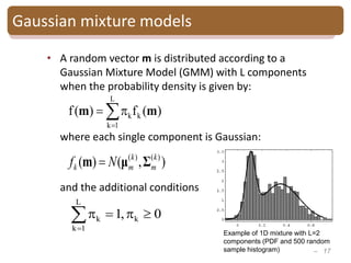
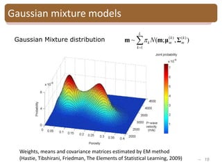
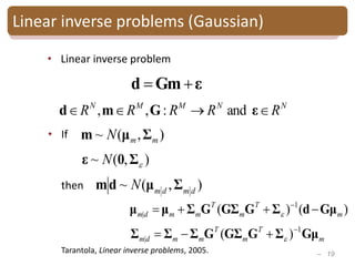
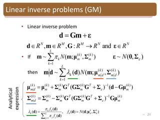
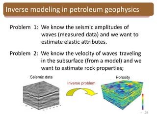
![– 30
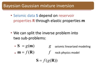
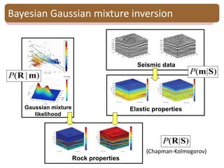
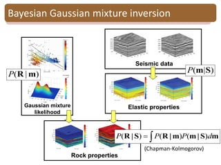
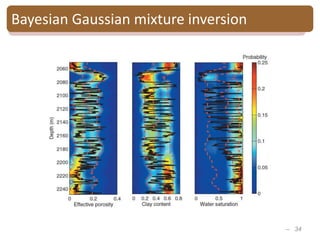
Bayesian Gaussian mixture inversion
• Goal: - Estimate reservoir properties R
from seismic data S
-Evaluate the model uncertainty
)](),(),([
],,[
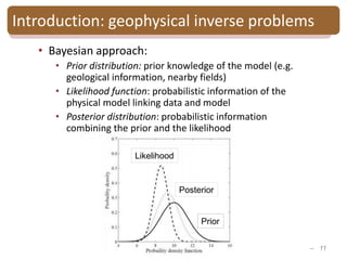
)|(
321
SSS
swc
P
S
R
SR
Porosity
Clay content
Water saturation
Partial-stack
seismic data
We estimate the posterior probability:](https://image.slidesharecdn.com/quebec-150403112446-conversion-gate01/85/Reservoir-Modeling-30-320.jpg)
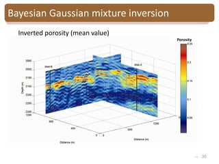
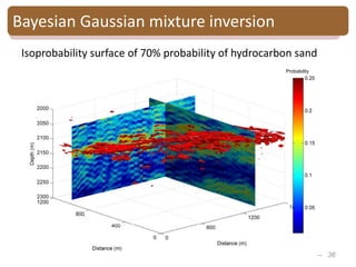
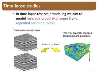
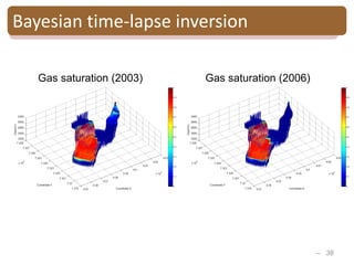
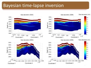
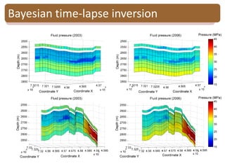
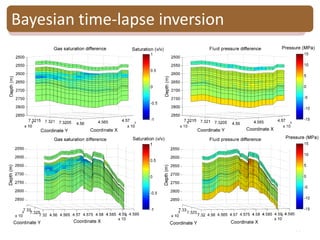
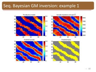
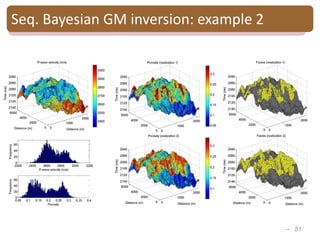
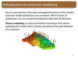
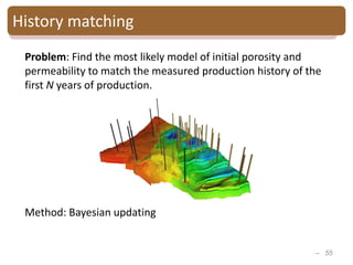
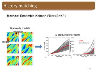

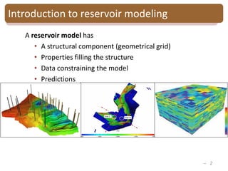
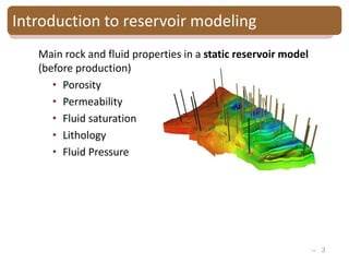
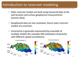
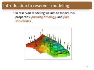
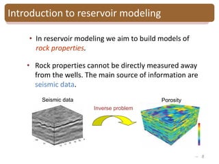
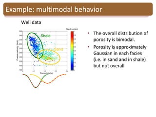
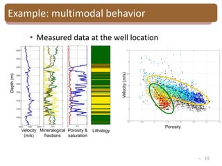
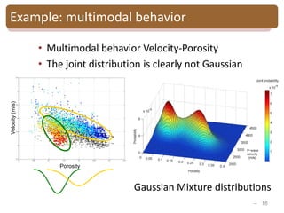
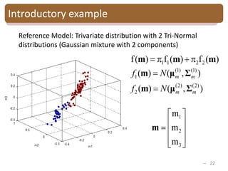
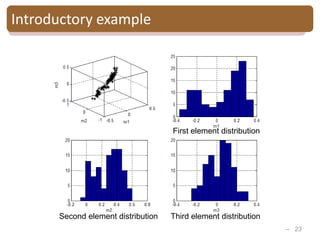
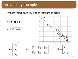
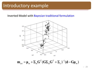
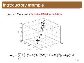
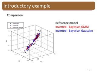
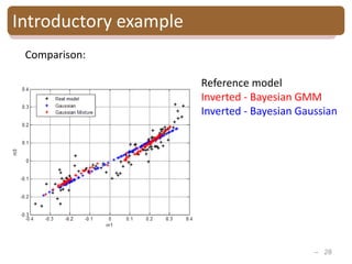
The document provides an introduction to Bayesian inverse theory and its applications in subsurface characterization and reservoir modeling. It discusses how Bayesian inversion can be used to estimate reservoir properties like porosity and saturation from seismic data by treating the inverse problem as estimating the posterior distribution given prior information and measurements. It also describes how the method can be extended to handle multimodal distributions using Gaussian mixture models. Further applications discussed include time-lapse inversion to estimate property changes over time and history matching to update reservoir models based on production data.


![Well Log Interpretation and Petrophysical Analisis in [Autosaved]](https://cdn.slidesharecdn.com/ss_thumbnails/a24a638f-02ab-4332-9396-89ba2cdd02b4-161128031018-thumbnail.jpg?width=640&height=640&fit=bounds)