22PCOAM16 ML Unit 3 notes PDF & QB. pdf

1. 22PCOAM16
MACHINE LEARNING
UNIT III NOTES & QB
B.TECH
III YEAR – V SEM (R22)
(2024-2025)
Prepared
By
Dr. M.Gokilavani
Department of Emerging Technologies
(Special Batch)

2. UNIT – III
Learning with Trees – Decision Trees – Constructing Decision Trees – Classification and Regression
Trees – Ensemble Learning – Boosting – Bagging – Different ways to Combine Classifiers – Basic
Statistics – Gaussian Mixture Models – Nearest Neighbor Methods – Unsupervised Learning – K means
Algorithms.
I. LEARNING WITH TREES:
 Learning refers to the process where algorithms, models, or systems adapt and improve their
performance based on data input and experience.
 “Tree" refers to a decision tree; a supervised learning algorithm used for both classification
and regression tasks.
 It's a flowchart-like structure where each node represents a test on an attribute, each branch
represents the outcome of the test, and each leaf node represents a class label or a predicted
value.
 Tree-based algorithms are a fundamental component of machine learning, offering intuitive
decision-making processes to human reasoning.
 These algorithms construct decision trees, where each branch represents a decision based on
features, ultimately leading to a prediction or classification.
 By recursively partitioning the feature space, tree-based algorithms provide transparent and
interpretable models, making them widely utilized in various applications.
What is Tree-based Algorithms?
 Tree-based algorithms are a class of supervised machine learning models that
construct decision trees to typically partition the feature space into regions, enabling a
hierarchical representation of complex relationships between input variables and output labels.
 Some of tree based algorithm are
i. Random forests
ii. Gradient Boosting techniques
iii. Decision trees
iv. Gini impurity
v. Information gain
How does Tree-based algorithm work?
The main four workflows of tree-based algorithms are discussed below:
1. Feature Splitting: Tree-based algorithms begin by selecting more informative features to
split a data set based on a specific criterion, such as Gini impurity or information gain etc.
2. Recursive splitting: The selected feature of dataset is used to split the data in two, and the
process is repeated for each resulting subset, forming a hierarchical binary tree structure.
This recursive splitting until stops a predefined criterion, like a maximum depth or a
minimum number of samples per train data, is met as long as it lasts.

3. 3. Leaf Node Function: As the tree grows, each terminal node (leaf) is given a predicted
outcome based on majority learning (for classification) or the sample value of that node of
the (for regression). This activates the tree to capture complex decision boundaries and
relationships in the data.
4. Ensemble Learning: For ensemble methods like Random Forests and Gradient Boosting
Machines, multiple trees are trained independently, and their predictions are combined to
obtain the final result. This group approach helps to reduce over fitting, increase
generalization, and improve overall model performance by combining the strengths of
individual trees and reducing their weaknesses.
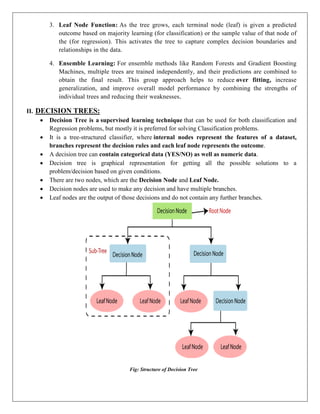
II. DECISION TREES:
 Decision Tree is a supervised learning technique that can be used for both classification and
Regression problems, but mostly it is preferred for solving Classification problems.
 It is a tree-structured classifier, where internal nodes represent the features of a dataset,
branches represent the decision rules and each leaf node represents the outcome.
 A decision tree can contain categorical data (YES/NO) as well as numeric data.
 Decision tree is graphical representation for getting all the possible solutions to a
problem/decision based on given conditions.
 There are two nodes, which are the Decision Node and Leaf Node.
 Decision nodes are used to make any decision and have multiple branches.
 Leaf nodes are the output of those decisions and do not contain any further branches.
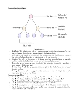
Fig: Structure of Decision Tree

4. Decision tree terminologies:
Fig: Decision Tree
 Root Node: This is the topmost node in a decision tree, representing the entire dataset. The root
node is where the first split occurs based on the most significant attribute.
 Leaf Node: A leaf node is the terminal node that represents the final classification or output. It
does not split further and provides the decision based on the previous splits.
 Splitting: This refers to the process of dividing a node into sub-nodes based on a certain
condition or attribute. Each split corresponds to a decision made by the model.
 Branch/Sub tree: A branch represents the subset of data that results from a split. It leads from a
parent node to a child node or leaf.
 Decision Node: A node that represents a decision to split the data further based on a particular
feature or attribute.
 Pruning: The process of removing parts of the tree that are not contributing to the model’s
accuracy in order to prevent over fitting.
Decision tree algorithm:
• Step-1: Begin the tree with the root node, says S, which contains the complete dataset.
• Step-2: Find the best attribute in the dataset using Attribute Selection Measure (ASM).
• Step-3: Divide the S into subsets that contains possible values for the best attributes.
• Step-4: Generate the decision tree node, which contains the best attribute.
• Step-5: Recursively make new decision trees using the subsets of the dataset created in step -3.
• Step-6: Continue this process until a stage is reached where you cannot further classify the nodes
and called the final node as a leaf node.

5. III. CONSTRUCTING DECISION TREES:
How is a Decision Tree Formed?
Building a decision tree involves several steps that ensure the final model is both accurate and
interpretable.
1. Selecting the Best Attribute
 The first step in building a decision tree is selecting the best attribute to split the dataset. This
is done using criteria such as
i. Information Gain
ii. Gini Index
i. Information Gain is based on the concept of entropy, which measures the amount of
disorder or uncertainty in the dataset.
 The goal is to select the attribute that reduces entropy the most when the data is
split.
 The formula for entropy is:
 Information gain is calculated as the difference between the entropy before and
after the split.
 The attribute with the highest information gain is selected as the splitting attribute.
ii. Gini index.
 The attribute that results in the highest gain (or lowest impurity) is chosen as the root
node.
 The Gini index measures the impurity of a dataset. A lower Gini index indicates a purer
dataset, meaning most of the instances belong to a single class.
 The Gini index is computed as:
 Attributes that result in the lowest Gini index after the split are considered the best
candidates for splitting the data.
2. Recursive Splitting
 Once the best attribute is selected, the data is split into subsets based on the value of that
attribute.
 This process is repeated recursively for each subset, creating branches and sub-branches until
the data is perfectly split or meets a stopping criterion (e.g., maximum depth or minimum
number of instances per leaf).
3. Stopping Criteria
 The decision tree continues splitting the data until one of the following conditions is met:
 All instances in a node belong to the same class.
 The maximum depth of the tree is reached.
 The number of instances in a node falls below a specified threshold.
4. Tree Pruning
• Pruning is a process of deleting the unnecessary nodes from a tree in order to get the
optimal decision tree.
• A too-large tree increases the risk of over fitting, and a small tree may not capture all the
important features of the dataset.

6. • Therefore, a technique that decreases the size of the learning tree without reducing accuracy is
known as Pruning.
• There are mainly two types of tree pruning technology used:
• Cost Complexity Pruning
• Reduced Error Pruning
TYPES OF DECISION TREE:
There are two types of decision tree:
1. ID3 Tree
2. Classification and Regression Tree (CART)
• ID3: This algorithm measures how mixed up the data is at a node using something
called entropy. It then chooses the feature that helps to clarify the data the most.
• CART: This algorithm uses a different measure called Gini impurity to decide how to split the
data. It can be used for both classification (sorting data into categories) and regression
(predicting continuous values) tasks.
IV. ID3(ITERATIVE DICHOTOMISER 3):
 The ID3 (Iterative Dichotomiser 3) algorithm was introduced by Ross Quinlan in 1986.
 It became a key development in the evolution of decision tree algorithms, influencing advanced
models like C4.5 and CART.
 The algorithm’s main contribution was its innovative use of entropy and information gain for
selecting the most informative attributes when splitting data.
Why Use Decision Trees?
There are various algorithms in Machine learning. Below are the two reasons for using the Decision
tree:
 Decision Trees usually mimic human thinking ability while making a decision, so it is easy to
understand.
 The logic behind the decision tree can be easily understood because it shows a tree-like
structure.
Purpose and Functionality:
The primary purpose of the ID3 algorithm is to construct a decision tree for classification tasks. It does
this by:
• Evaluating each attribute in the dataset to determine its potential to reduce uncertainty
(measured using entropy).
• Selecting the attribute with the highest information gain to create splits that maximize
classification accuracy.
• Repeating the process recursively on smaller subsets until the tree fully classifies the data.
The ID3 algorithm is particularly effective with categorical data and is considered a foundational
method in machine learning for its simplicity and logical approach.

7. STEPS IN ID3 ALGORITHM:
The ID3 algorithm constructs a decision tree by recursively splitting the dataset based on the attribute
that provides the highest information gain.
Step 1: Calculate the Entropy of the Dataset
• Entropy measures the impurity or randomness in the dataset.
The formula for entropy is:
Where pi is the proportion of instances belonging to class i.
Step 2: Compute Information Gain for Each Attribute
• Information Gain is the reduction in entropy after splitting the dataset based on an attribute.
The formula for information gain is:
Here, Sv is the subset of S for which attribute A has value V .
Step 3: Select the Attribute with the Highest Information Gain
• Choose the attribute that most effectively reduces uncertainty and use it as the decision node.
Step 4: Split the Dataset
• Partition the dataset into subsets based on the selected attribute’s values.
• Assign branches for each possible outcome of the attribute.
Step 5: Recursively Apply the Process
• Repeat steps 1 to 4 for each subset, excluding the previously used attribute.
• Continue until one of the following termination conditions is met:
• All instances in a subset belong to the same class.
• There are no remaining attributes to split.
• The dataset is empty.
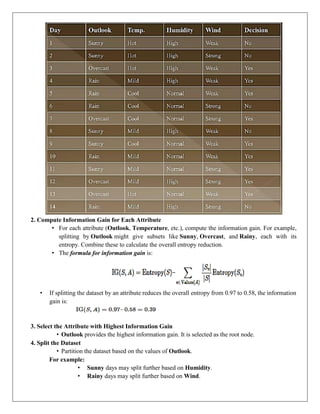
EXAMPLE: ID Dataset
Imagine a dataset with attributes like Outlook, Temperature, Humidity, and Wind. The target variable is
whether to Play Tennis (Yes/No).
1. Calculate Entropy of the Dataset
• The dataset contains records of days when tennis was played or not. Calculate the entropy for
the target variable Play Tennis:
• The formula for entropy is:
In given Example, a dataset has 10 instances, with 6 labeled “Yes” and 4 labeled “No”.

8. 2. Compute Information Gain for Each Attribute
• For each attribute (Outlook, Temperature, etc.), compute the information gain. For example,
splitting by Outlook might give subsets like Sunny, Overcast, and Rainy, each with its
entropy. Combine these to calculate the overall entropy reduction.
• The formula for information gain is:
• If splitting the dataset by an attribute reduces the overall entropy from 0.97 to 0.58, the information
gain is:
3. Select the Attribute with Highest Information Gain
• Outlook provides the highest information gain. It is selected as the root node.
4. Split the Dataset
• Partition the dataset based on the values of Outlook.
For example:
• Sunny days may split further based on Humidity.
• Rainy days may split further based on Wind.

9. 5. Repeat the Process Recursively
• Apply the same steps to the subsets until all records are classified or no further splits are
possible.
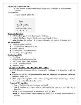
6. Visualization
Role in ID3 Algorithm:
• Calculate Entropy: Compute the entropy for the dataset.
• Evaluate Attributes: Compute the information gain for each attribute.
• Select Attribute: The attribute with the highest information gain becomes the decision node.
Advantage of ID3:
• Simplicity and Interpretability
• Efficient Handling of Categorical Data
• Greedy Approach
• Foundation for Advanced Algorithms
• Versatility Across Applications
Disadvantage of ID3:
• Over fitting
• Difficulty Handling Continuous Data
• Bias Towards Multi-Valued Attributes
• Lack of Pruning Mechanisms
• Scalability Issues
V. CLASSIFICATION AND REGRESSION TREES:
 CART: This algorithm uses a different measure called Gini impurity to decide how to split the
data.
 It can be used for both classification (sorting data into categories) and regression (predicting
continuous values) tasks.
 CART is a predictive algorithm used in Machine learning and it explains how the target variable’s
values can be predicted based on other matters.
Steps in CART algorithm:
• Step 1: The best split point of each input is obtained.
• Step 2: Based on the best split points of each input in Step 1, the new “best” split point is
identified.
• Step 3: Split the chosen input according to the “best” split point.
• Step 4: Continue splitting until a stopping rule is satisfied or no further desirable splitting is
available.

10. GINI Index:
• It is a measure of impurity (non-homogeneity) widely used in decision trees.
• It aims to measure the probability of misclassifying a randomly chosen element from the
dataset.
• The greater the value of the Gini Index, the greater the chances of having misclassifications.
Formula to calculate the Gini Index is calculated using the formula:
Where p ( j | t ) is the relative frequency of class j at node t.
• The maximum value is (1 – 1/n) indicating that n classes are equally distributed.
• The minimum value is 0 indicating that all records belong to a single class.
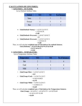
EXAMPLE: CART DATASET

11. CALCULATION OF GINI INDEX:
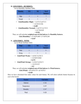
i. GINI INDEX – OUTLOOK:
Let us Outlook Attribute Table:
 Gini(Outlook=Sunny) = 1-(2/5)^2-(3/5)^2
= 1-0.16-0.36
= 0.48
 Gini(Outlook=Overcast) = 1-(4/4)^2-(0/4)^2
= 0
 Gini(Outlook=Overcast) = 1-(3/5)^2-(2/5)^2
= 1-0.36-0.16
= 0.48
Then, we will calculate weighted sum of Gini indexes for outlook features.
Gini (Outlook) = (5/14)*0.48-(4/4)*0+(5/14)*0.48
= 0.171+0+0.171
= 0.342
ii. GINI INDEX – TEMPARATURE:
Let us Temperature Attribute Table:
• Gini(Temp=Hot) = 1-(2/4)^2-(2/4)^2
= 0.5
• Gini(Temp=Cool) = 1-(3/4)^2-(1/4)^2
= 0.5625-0.0625
= 0.375
• Gini(Temp=Mild) = 1-(4/6)^2-(2/6)^2
= 1-0.444-0.111
= 0.445
Then, we will calculate weighted sum of Gini indexes for Temperature features.
Gini (Temp) = (4/14)*0.5 + (4/14)*0.375 + (6/14)*0.445
= 0.145+0.107+0.190
= 0.439

12. iii. GINI INDEX – HUMIDITY:
Let us Humidity Attribute Table:
• Gini(Humidity=High) = 1-(3/7)^2-(4/7)^2
= 1-0.183-0.326
= 0.489
• Gini(Humidity=Normal) =1-(6/7)^2-(1/7)^2
=1-0.734-0.02
= 0.244
Then, we will calculate weighted sum of Gini indexes for Humidity features.
Gini (Humidity) = (7/14)*0.489+ (7/14)*0.244
= 0.367
iv. GINI INDEX – WIND:
Let us Wind Attribute Table:
• Gini(Wind=Weak) = 1-(6/8)^2-(2/8)^2
= 1-0.5625-0.062
= 0.375
• Gini(Wind=Strong) = 1-(3/6)^2-(3/6)^2
= 1-0.25-0.25
= 0.5
Then, we will calculate weighted sum of Gini indexes for Wind features.
Gini (Wind) = (8/14)*0.375+ (6/14)*0.5
= 0.428
Here we have calculated Gini index values for each feature. We will select outlook feature because its
cost is the lowest.

13. Solution: Decision Tree for attribute Outlook, Temperature, Humidity, wind attribute as,

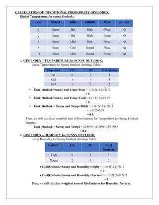
14. CALCULATION OF CONDITIONAL PROBABILITY GINI INDEX:
Gini of Temperature for sunny Outlook:
i. GINI INDEX – TEMPARETURE for SUNNY OUTLOOK:
Let us Temperature for Sunny Outlook Attribute Table:
• Gini (Outlook=Sunny and Temp=Hot) = 1-(0/2)^2-(2/2)^2
= 0
• Gini (Outlook=Sunny and Temp=Cool) =1-(1/1)^2-(0/1)^2
= 0
• Gini (Outlook = Sunny and Temp=Mild) = 1-(1/2)^2-(1/2)^2
= 1-0.25-0.25
= 0.5
Then, we will calculate weighted sum of Gini indexes for Temperature for Sunny Outlook
features.
Gini (Outlook = Sunny and Temp) = (2/5)*0+ (1/5)*0+ (2/5)*0.5
= 0.2
ii. GINI INDEX – HUMIDITY for SUNNY OUTLOOK:
Let us Humidity for Sunny Outlook Attribute Table:
 Gini(Outlook=Sunny and Humidity=High) = 1-(0/3)^2-(3/3)^2
= 0
 Gini(Outlook=Sunny and Humidity=Normal) =1-(2/2)^2-(0/2)^2
= 0
Then, we will calculate weighted sum of Gini indexes for Humidity features.

15. Gini (Outlook=Sunny and Humidity) = (3/5)*0+ (2/5)*0
= 0
iii. GINI INDEX – WINDY for SUNNY OUTLOOK:
Let us Windy for Sunny Outlook Attribute Table:
 Gini (Outlook=Sunny and Wind=Weak) = 1-(1/3)^2-(2/)^2
= 0.266
 Gini(Outlook Sunny and Wind=Strong) =1-(1/2)^2-(1/2)^2
= 0.2
Then, we will calculate weighted sum of Gini indexes for Wind for Sunny Outlook features.
Gini (Outlook=Sunny and Humidity) = (3/5)*0.266 + (2/5)*0.2
= 0.466
Here we have calculated Gini index values for each feature. We will select outlook feature because its
cost is the lowest.
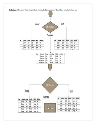
Solution:

16. VI. ENSEMBLE LEARNING:
 Ensemble learning is a technique in machine learning that combines the predictions from
multiple individual models to achieve better predictive performance than any single model
alone.
 The fundamental idea is to leverage the strengths and compensate for the weaknesses of various
models by aggregating their predictions.
Types of Ensemble Learning:
There are two main types of ensemble methods:
i. Bagging (Bootstrap Aggregating): Models are trained independently on different subsets of
the data, and their results are averaged or voted on.
ii. Boosting: Models are trained sequentially, with each one learning from the mistakes of the
previous model.
BOOSTING & BAGGING:
i. BAGGING ALGORITHM:
 Bootstrap aggregating also known as bagging, is a machine learning ensemble dataset
designed to improve the stability and accuracy of machine learning algorithms used in
statistical classification and regression.
 It decreases the variance and helps to avoid over fitting.
 It is usually applied to decision tree methods.
 Bagging is a special case of the model averaging approach.
Description of the technique:
• Suppose a set D of d tuples, at each iteration ith
, a training set Di of d tuples is selected via
row sampling with a replacement method (i.e., there can be repetitive elements from
different d tuples) from D (i.e., bootstrap).
• Then a classifier model Mi is learned for each training set D < i.
• Each classifier Mi returns its class prediction.
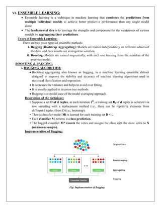
• The bagged classifier M* counts the votes and assigns the class with the most votes to X
(unknown sample).
Implementation of Bagging:
Fig: Implementation of Bagging

17. • Step 1: Multiple subsets are created from the original data set with equal tuples, selecting
observations with replacement.
• Step 2: A base model is created on each of these subsets.
• Step 3: Each model is learned in parallel with each training set and independent of each
other.
• Step 4: The final predictions are determined by combining the predictions from all the
models.
Bagging Algorithm:
Bagging Classifier:
• Bagging or Bootstrap aggregating is a type of ensemble learning in which multiple base
models are trained independently and parallel on different subsets of training data.
• In bagging classifier, the final prediction is made by aggregating the predictions of all
base models using majority voting.
• In the models of regression the final prediction is made by averaging the predictions of the
all base model and that is known as bagging regression.
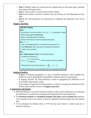
ii. BOOSTING METHOD:
 Bootstrap Method is a powerful statistical technique widely used in mathematics for estimating
the distribution of a statistic by resampling with replacement from the original data.
 The bootstrap method is a resampling technique that allows you to estimate the properties
of an estimator (such as its variance or bias) by repeatedly drawing samples from the original
data.
 It was introduced by Bradley Efron in 1979 and has since become a widely used tool in
statistical inference.

18.  The bootstrap method is useful in situations where the theoretical sampling distribution of a
statistic is unknown or difficult to derive analytically.
 Bootstrapping is a statistical procedure that resample's a single data set to create many
simulated samples.
 Bootstrap Method or Bootstrapping is a statistical procedure that resample's a single
data set to create many simulated samples.
 This process allows for, "calculation of standard errors, confidence intervals, and
hypothesis testing” according to a post on bootstrapping statistics from statistician Jim Frost.
 It can be used to estimate summary statistics such as the mean and standard deviation.
 Bootstrap Method or Bootstrapping is a statistical technique for estimating an entire
population quantity by averaging estimates from multiple smaller data samples.
Fig: Boosting Method
Implementation of Boosting Method:
The procedure can be summarized as follows:
Step 1: Choose the number of bootstrap samples to take.
Step 2: Choose your sample size for each bootstrap sample, draw a replacement sample of the
size you selected.
Step 3: Calculate the statistics for the samples calculate the average of the computed sample
statistics.
Example:
• The Random Forest model uses Bagging, where decision tree models with higher variance are
present.
• It makes random feature selection to grow trees.
• Several random trees make a Random Forest.

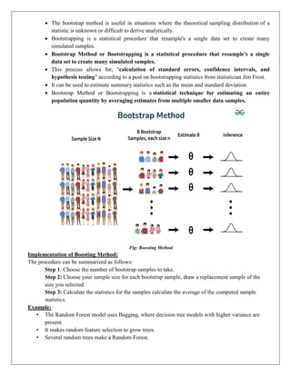
19. Boosting Algorithm:
• Step 1: Initialize the dataset and assign equal weight to each of the data point.
• Step 2: Provide this as input to the model and identify the wrongly classified data points.
• Step 3: Increase the weight of the wrongly classified data points and decrease the weights of
correctly classified data points. And then normalize the weights of all data points.
• Step 4: if (got required results)
Goto step 5
else
Goto step 2
• Step 5: End
Implementation of Boosting Algorithm:
Fig: Implementation of Boosting Algorithm
• Step 1: Initially, a model is built using the training data.
• Step 2: Subsequent models are then trained to address the mistakes of their predecessors.
• Step 3: Boosting assigns weights to the data points in the original dataset.
• Step 4: Higher weights: Instances that were misclassified by the previous model receive higher
weights.
• Step 5: Lower weights: Instances that were correctly classified receive lower weights.

20. • Step 6: Training on weighted data: The subsequent model learns from the weighted dataset,
focusing its attention on harder-to-learn examples (those with higher weights).
• Step 7: This iterative process continues until:
• The entire training dataset is accurately predicted, or
• A predefined maximum number of models are reached.
Advantages of Boosting Algorithm:
• Improved Accuracy: By combining multiple weak learners it enhances predictive accuracy for
both classification and regression tasks.
• Robustness to over fitting: Unlike traditional models it dynamically adjusts weights to prevent
over fitting.
• Handles Imbalanced Data Well: It prioritizes misclassified points making it effective for
imbalanced datasets.
• Better Interpretability: The sequential nature of helps break down decision-making making the
model more interpretable.
VII. DIFFERENT WAYS TO COMBINE CLASSIFIERS:
 Classification teaches a machine to sort things into categories.
 It learns by looking at examples with labels (like emails marked “spam” or “not spam”).
 After learning, it can decide which category new items belong to, like identifying if a new
email is spam or not.
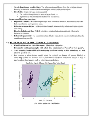
 For example a classification model might be trained on dataset of images labeled as
either dogs or cats and it can be used to predict the class of new and unseen images as dogs or
cats based on their features such as color, texture and shape.
Fig: Getting started with Classification

21.  Explaining classification in ml, horizontal axis represents the combined values of color and
texture features.
 Vertical axis represents the combined values of shape and size features.
 Each colored dot in the plot represents an individual image, with the color indicating whether
the model predicts the image to be a dog or a cat.
 The shaded areas in the plot show the decision boundary, which is the line or region that the
model uses to decide which category (dog or cat) an image belongs to.
 The model classifies images on one side of the boundary as dogs and on the other side as cats,
based on their features.
Need of classifier:
• A classifier in machine learning is an algorithm that automatically orders or categorizes data into
one or more of a set of “classes.”
• The process of categorizing or classifying information based on certain characteristics is known as
classification.
• Classifiers are typically used in supervised learning systems where the correct class for each input
example is known during training.
• The goal of a classifier is to learn from the training data and be able to make accurate predictions on
unseen data.
Types of classifiers:
There are three types of classifier:
i. Binary Classifier
ii. Multiclass classifier
iii. Multilabel classifier
i. Binary Classifiers:
 These are used when there are only two possible classes.
 For example, an email classifier might be designed to detect spam and non-spam
emails.
 This is the simplest kind of classification. In binary classification, the goal is to sort
the data into two distinct categories.
 Imagine a system that sorts emails into either spam or not spam.
 It works by looking at different features of the email like certain keywords or
sender details, and decides whether it’s spam or not.
 It only chooses between these two options.
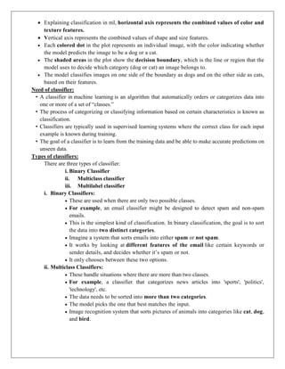
ii. Multiclass Classifiers:
 These handle situations where there are more than two classes.
 For example, a classifier that categorizes news articles into 'sports', 'politics',
'technology', etc.
 The data needs to be sorted into more than two categories.
 The model picks the one that best matches the input.
 Image recognition system that sorts pictures of animals into categories like cat, dog,
and bird.

22.  Basically, machine looks at the features in the image (like shape, color, or
texture) and chooses which animal the picture is most likely to be based on the
training it received.
Fig: Binary classification Vs Multi class classification
iii. Multilabel Classifiers:
 These can assign multiple labels to each instance. For example, a movie could be
classified into multiple genres like 'comedy', 'drama', and 'action' simultaneously.
 In multi-label classification single piece of data can belong to multiple
categories at once.
 Unlike multiclass classification where each data point belongs to only one class,
multi-label classification allows data points to belong to multiple classes.
 A movie recommendation system could tag a movie as both action and comedy.
 The system checks various features (like movie plot, actors, or genre tags) and
assigns multiple labels to a single piece of data, rather than just one.
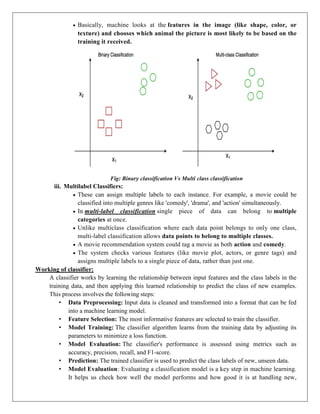
Working of classifier:
A classifier works by learning the relationship between input features and the class labels in the
training data, and then applying this learned relationship to predict the class of new examples.
This process involves the following steps:
• Data Preprocessing: Input data is cleaned and transformed into a format that can be fed
into a machine learning model.
• Feature Selection: The most informative features are selected to train the classifier.
• Model Training: The classifier algorithm learns from the training data by adjusting its
parameters to minimize a loss function.
• Model Evaluation: The classifier's performance is assessed using metrics such as
accuracy, precision, recall, and F1-score.
• Prediction: The trained classifier is used to predict the class labels of new, unseen data.
• Model Evaluation: Evaluating a classification model is a key step in machine learning.
It helps us check how well the model performs and how good it is at handling new,

23. unseen data. Depending on the problem and needs we can use different metrics to
measure its performance.
Fig: Classification Machine learning
 If the quality metric is not satisfactory, the ML algorithm or hyper parameters can be
adjusted, and the model is retrained.
 This iterative process continues until a satisfactory performance is achieved.
 In short, classification in machine learning is all about using existing labeled data to teach
the model how to predict the class of new, unlabeled data based on the patterns it has
learned.
Examples of Machine Learning Classification in Real Life:
Classification algorithms are widely used in many real-world applications across various
domains, including:
i. Email spam filtering
ii. Credit risk assessment: Algorithms predict whether a loan applicant is likely to default by
analyzing factors such as credit score, income, and loan history. This helps banks make
informed lending decisions and minimize financial risk.
iii. Medical diagnosis: Machine learning models classify whether a patient has a certain
condition (e.g., cancer or diabetes) based on medical data such as test results, symptoms,
and patient history. This aids doctors in making quicker, more accurate diagnoses,
improving patient care.
iv. Image classification: Applied in fields such as facial recognition, autonomous driving, and
medical imaging.
v. Sentiment analysis: Determining whether the sentiment of a piece of text is positive,
negative, or neutral. Businesses use this to understand customer opinions, helping to
improve products and services.

24. vi. Fraud detection: Algorithms detect fraudulent activities by analyzing transaction patterns
and identifying anomalies crucial in protecting against credit card fraud and other financial
crimes.
vii. Recommendation systems : Used to recommend products or content based on past user
behavior, such as suggesting movies on Netflix or products on Amazon. This
personalization boosts user satisfaction and sales for businesses.
Classification Modeling in Machine Learning
 The fundamentals of classification, it’s time to explore how we can use these concepts
to build classification models. Classification modeling refers to the process of using machine
learning algorithms to categorize data into predefined classes or labels.
 These models are designed to handle both binary and multi-class classification tasks,
depending on the nature of the problem.
 Let’s see key characteristics of Classification Models:
1. Class Separation: Classification relies on distinguishing between distinct classes. The
goal is to learn a model that can separate or categorize data points into predefined
classes based on their features.
2. Decision Boundaries: The model draws decision boundaries in the feature space to
differentiate between classes. These boundaries can be linear or non-linear.
3. Sensitivity to Data Quality: Classification models are sensitive to the quality and
quantity of the training data. Well-labeled, representative data ensures better
performance, while noisy or biased data can lead to poor predictions.
4. Handling Imbalanced Data: Classification problems may face challenges when one
class is underrepresented. Special techniques like resampling or weighting are used to
handle class imbalances.
5. Interpretability: Some classification algorithms, such as Decision Trees, offer higher
interpretability, meaning it’s easier to understand why a model made a particular
prediction.
Classification Algorithms
 Implementation of any classification model it is essential to understand Logistic Regression,
which is one of the most fundamental and widely used algorithms in machine learning for
classification tasks.
 There are various types of classifiers algorithms.
i. Linear Classifiers: Linear classifier models create a linear decision boundary between
classes. They are simple and computationally efficient. Some of the
linear classification models are as follows:
 Logistic Regression
 Support Vector Machines having kernel = ‘linear’
 Single-layer Perception
 Stochastic Gradient Descent (SGD) Classifier
ii. Non-linear Classifiers: Non-linear models create a non-linear decision boundary
between classes. They can capture more complex relationships between input features
and target variable. Some of the non-linear classification models are as follows:
 K-Nearest Neighbors

25.  Kernel SVM
 Naive Bayes
 Decision Tree Classification
 Ensemble learning classifiers:
 Random Forests,
 AdaBoost,
 Bagging Classifier,
 Voting Classifier,
 Extra Trees Classifier
 Multi-layer Artificial Neural Networks
VIII. BASIC STATISTICS:
 Statistics is the science of collecting, organizing, analyzing, interpreting, and presenting
data.
 It encompasses a wide range of techniques for summarizing data, making inferences, and
drawing conclusions.
 Statistical methods help quantify uncertainty and variability in data, allowing researchers and
analysts to make data-driven decisions with confidence.
Types of Statistics:
There are commonly two types of statistics, which are discussed below:
 Descriptive Statistics: "Descriptive Statistics" helps us simplify and organize big
chunks of data. This makes large amounts of data easier to understand.
 Inferential Statistics: "Inferential Statistics" is a little different. It uses smaller data
to draw conclusions about a larger group. It helps us predict and draw conclusions
about a population.
1. DESCRIPTIVE STATISTICS:
 Descriptive statistics summarize and describe the features of a dataset, providing a foundation for
further statistical analysis.
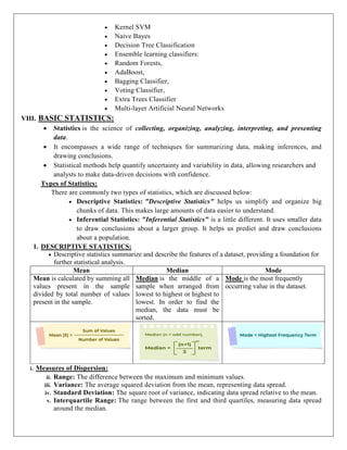
Mean Median Mode
Mean is calculated by summing all
values present in the sample
divided by total number of values
present in the sample.
Median is the middle of a
sample when arranged from
lowest to highest or highest to
lowest. In order to find the
median, the data must be
sorted.
Mode is the most frequently
occurring value in the dataset.
i. Measures of Dispersion:
ii. Range: The difference between the maximum and minimum values.
iii. Variance: The average squared deviation from the mean, representing data spread.
iv. Standard Deviation: The square root of variance, indicating data spread relative to the mean.
v. Interquartile Range: The range between the first and third quartiles, measuring data spread
around the median.

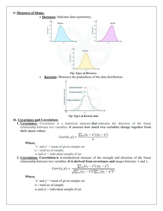
26. iv.Measures of Shape:
 Skewness: Indicates data asymmetry.
Fig: Types of Skewness
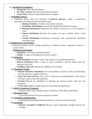
 Kurtosis: Measures the peakedness of the data distribution.
Fig: Types of Kurtosis data
iii. Covariance and Correlation:
1. Covariance: Covariance is a statistical measure that indicates the direction of the linear
relationship between two variables. It assesses how much two variables change together from
their mean values.
Where,
‘x’ and y’ = mean of given sample set
n = total no of sample
xi and yi = individual sample of set
2. Correlation: Correlation is a standardized measure of the strength and direction of the linear
relationship between two variables. It is derived from covariance and ranges between -1 and 1.
Where,
‘x’ and y’ = mean of given sample set
n = total no of sample
xi and yi = individual sample of set

27. iv. Visualization Techniques:
 Histograms: Show data distribution.
 Box Plots: Highlight data spread and potential outliers.
 Scatter Plots: Illustrate relationships between variables.
v. Probability Theory:
 Probability theory forms the backbone of statistical inference, aiding in quantifying
uncertainty and making predictions based on data.
i. Random Variables: Variables with random outcomes.
ii. Probability Distributions: Describe the likelihood of different outcomes.
iii. Binomial Distribution: Represents the number of successes in a fixed number of
trials.
iv. Poisson distribution: Describes the number of events occurring within a fixed
interval.
v. Normal Distribution: Characterizes continuous data symmetrically distributed
around the mean.
2. INFERENTIAL STATISTICS
 Inferential statistics involve making predictions or inferences about a population based on a
sample of data.
i. Population and Sample:
 Population: The entire group being studied.
 Sample: A subset of the population used for analysis.
ii. Estimation:
 Point Estimation: Provides a single value estimate of a population parameter.
 Interval Estimation: Offers a range of values (confidence interval) within which the
parameter likely lies.
 Confidence Intervals: Indicate the reliability of an estimate.
iii. Hypothesis Testing:
 Null and Alternative Hypotheses: The null hypothesis assumes no effect or relationship,
while the alternative suggests otherwise.
 Type I and Type II Errors: Type I error is rejecting a true null hypothesis, while Type II
is failing to reject a false null hypothesis.
 P-Values: Measure the probability of obtaining the observed results under the null
hypothesis.
 T-Tests and z-Tests: Compare means to assess statistical significance.
iv.ANOVA (Analysis of Variance):
Compares means across multiple groups to determine if they differ significantly.
v. Chi-Square Tests:
Assess the association between categorical variables.
vi. Correlation and Regression:
Understanding relationships between variables is critical in machine learning.
vii. Correlation
 Pearson Correlation Coefficient: Measures linear relationship strength between two
variables.

28.  Spearman Rank Correlation: Assesses the strength and direction of the monotonic
relationship between variables.
viii. Regression Analysis
 Simple Linear Regression: Models the relationship between two variables.
 Multiple Linear Regression: Extends to multiple predictors.
 Assumptions of Linear Regression: Linearity, independence, homoscedasticity,
normality.
 Interpretation of Regression Coefficients: Explains predictor influence on the
response variable.
 Model Evaluation Metrics: R-squared, Adjusted R-squared, RMSE.
ix.Bayesian Statistics
 Bayesian statistics incorporate prior knowledge with current evidence to update beliefs.
 Bayes' Theorem is a fundamental concept in probability theory that relates conditional
probabilities. It is named after the Reverend Thomas Bayes, who first introduced the
theorem.
 Bayes' Theorem is a mathematical formula that provides a way to update probabilities
based on new evidence.
 The formula is as follows:
P (A∣B) = P (B) P (B∣A) ⋅ P(A),
Where
 P (A∣B): The probability of event A given that event B has occurred (posterior
probability).
 P (B∣A): The probability of event B given that event A has occurred
(likelihood).
 P (A): The probability of event A occurring (prior probability).
 P (B): The probability of event B occurring.
IX. GAUSSIAN MIXTURE MODELS:
 Clustering is a key technique in unsupervised learning, used to group similar data points
together.
 While traditional methods like K-Means and Hierarchical Clustering are widely used, they
assume that clusters are well-separated and have rigid shapes. This can be limiting in real-
world scenarios where clusters can be more complex.
 To overcome these limitations, Gaussian Mixture Models (GMM) offers a more flexible
approach.
 Unlike K-Means, which assigns each point to a single cluster, GMM uses a probabilistic
approach to cluster the data, allowing clusters to have more varied shapes and soft boundaries.
Gaussian Mixture Model Vs K-Means:
 A Gaussian mixture model is a soft clustering technique used in unsupervised learning to
determine the probability that a given data point belongs to a cluster.
 It’s composed of several Gaussians, each identified by k ∈ {1… K}, where K is the number of
clusters in a data set and is comprised of the following parameters.

29.  K-means is a clustering algorithm that assigns each data point to one cluster based on the
closest centroid.
 It’s a hard clustering method, meaning each point belongs to only one cluster with no
uncertainty.
 On the other hand, Gaussian Mixture Models (GMM) use soft clustering, where data points
can belong to multiple clusters with a certain probability. This provides a more flexible and
nuanced way to handle clusters, especially when points are close to multiple centroids.
How Gaussian Mixture Models Work?
 GMM actually works, where the clustering process relies solely on the centroid and assigns
each data point to one cluster, GMM uses a probabilistic approach. Here’s how GMM
performs clustering:
1. Multiple Gaussians (Clusters): Each cluster is represented by a Gaussian distribution,
and the data points are assigned probabilities of belonging to different clusters based on
their distance from each Gaussian.
2. Parameters of a Gaussian: The core of GMM is made up of three main parameters for
each Gaussian:
 Mean (μ): The center of the Gaussian distribution.
 Covariance (Σ): Describes the spread or shape of the cluster.
 Mixing Probability (π): Determines how dominant or likely each cluster is in
the data.
 The Gaussian mixture model assigns a probability to each data point xnx_nxnof belonging to a
cluster. The probability of data point coming from Gaussian cluster k is expressed as
Where,
 znzn=k is a latent variable indicating which Gaussian the point belongs to.
 πkπk is the mixing probability of the k-th Gaussian.
 N(xn∣μk,Σk)N(xn∣μk,Σk)is the Gaussian distribution with mean μkmu_kμk and
covariance Σk
The Expectation-Maximization (EM) Algorithm:
 To fit a Gaussian Mixture Model to the data, we use the Expectation-Maximization
(EM) algorithm, which is an iterative method that optimizes the parameters of the Gaussian
distributions (mean, covariance, and mixing coefficients).
 It works in two main steps:
1. Expectation Step (E-step):
 In this step, the algorithm calculates the probability that each data point belongs to
each cluster based on the current parameter estimates (mean, covariance, mixing
coefficients).
2. Maximization Step (M-step):
 After estimating the probabilities, the algorithm updates the parameters (mean,
covariance, and mixing coefficients) to better fit the data.

30. These two steps are repeated until the model converges, meaning the parameters no longer change
significantly between iterations.
GMM Works:
 Initialization: Start with initial guesses for the means, covariances, and mixing coefficients
of each Gaussian distribution.
 E-step: For each data point, calculate the probability of it belonging to each Gaussian
distribution (cluster).
 M-step: Update the parameters (means, covariance’s, mixing coefficients) using the
probabilities calculated in the E-step.
 Repeat: Continue alternating between the E-step and M-step until the log-likelihood of the
data (a measure of how well the model fits the data) converges.
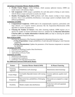
Implementation of GMM in python:
Let’s take a simple example using the Iris dataset and fit a Gaussian Mixture Model with 3 clusters
 Dataset: We use only two features: sepal length and sepal width.
 Fitting the Model: We fit the data as a mixture of 3 Gaussians.
 Result: The model assigns each data point to a cluster based on the probabilities.
After convergence, the GMM model will have updated the parameters to best fit the data.
Fig: GMM Clustering
 This scatter plot shows the result of clustering data using a Gaussian Mixture Model (GMM).
 The data points represent measurements of flower species based on sepal length and sepal
width.
 The points are divided into three clusters, represented by different colors (yellow, purple, and
teal), which indicate that GMM has identified three distinct groups within the data.

31. Advantages of Gaussian Mixture Models (GMM):
 Flexible Cluster Shapes: Unlike K-Means, which assumes spherical clusters, GMM can
model clusters with arbitrary shapes.
 Soft Assignment: GMM assigns a probability for each data point to belong to each cluster,
while K-Means assigns each point to exactly one cluster.
 Handles Overlapping Data: GMM performs well when clusters overlap or have varying
densities. Since it uses probability distributions, it can assign a point to multiple clusters with
different probabilities.
Limitations of GMM:
 Computational Complexity: GMM tends to be computationally expensive, particularly with
large datasets, as it requires iterative processes like the Expectation-Maximization (EM)
algorithm to estimate the parameters.
 Choosing the Number of Clusters: Like other clustering methods, GMM requires you to
specify the number of clusters beforehand. However, methods like the Bayesian Information
Criterion (BIC) and Akaike Information Criterion (AIC) can help in selecting the optimal
number of clusters based on the data.
Role of EM in GMM:
EM finds the parameters of the Gaussian components by alternating between two steps:
 E-Step (Expectation): Assigns probabilities of each data point belonging to each Gaussian
component.
 M-Step (Maximization): Updates the parameters of the Gaussian components to maximize
the likelihood.
Advantages of GMM:
1. Flexibility in Modeling Complex Data Distributions
2. Soft Clustering Capabilities
3. Applicability to Diverse Fields
Limitations of GMM:
1. Sensitivity to Initialization
2. Computational Complexity
3. Challenges with High-Dimensional Data.
Key Differences between GMM and K-Means:
Feature Gaussian Mixture Model (GMM) K-Means Clustering
Clustering
Approach
Probabilistic (soft clustering) Deterministic (hard clustering)
Cluster Shape
Can handle ellipsoidal clusters with varying
sizes
Assumes spherical, equally-sized
clusters
Assignment
Data points have probabilities of belonging
to clusters
Data points are assigned to a single
cluster
Flexibility Models complex data distributions
Works best with well-separated,
simple data

32. Parameters
Incorporates means, covariance, and mixing
coefficients
Only considers cluster centroids
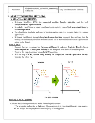
X. NEAREST NEIGHBOR METHODS:
K MEANS ALGORITHMS:
 K-Nearest Neighbors (kNN) is a supervised machine learning algorithm used for both
classification and regression tasks.
 It works by classifying a new data point based on the majority class of its k nearest neighbors in
the training dataset.
 The algorithm's simplicity and ease of implementation make it a popular choice for various
applications.
 K-Nearest Neighbors is also called as a lazy learner algorithm because it does not learn from the
training set immediately instead it stores the dataset and at the time of classification it performs an
action on the dataset.
Need of KNN:
• Supports there are two categories. Category A (Cluster 1) category B (cluster 2) and w have a
new data point X1 (K point from dataset), so this data point lie in which of these categories.
• To solve this type of problem, we need a KNN algorithm.
• With the help of KNN, we can easily identify the category or class of a particular dataset.
Consider the below Fig.
Fig: KNN Algorithm
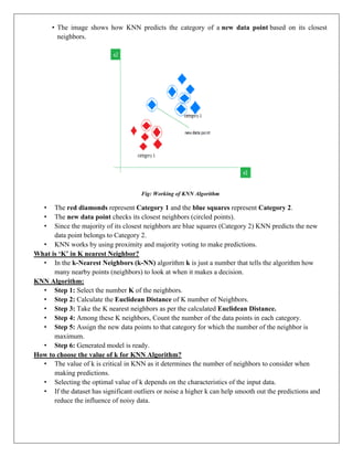
Working of KNN Algorithm:
Consider the following table of data points containing two features:
• The new point is classified as Category 2 because most of its closest neighbors are blue squares.
• KNN assigns the category based on the majority of nearby points.

33. • The image shows how KNN predicts the category of a new data point based on its closest
neighbors.
Fig: Working of KNN Algorithm
• The red diamonds represent Category 1 and the blue squares represent Category 2.
• The new data point checks its closest neighbors (circled points).
• Since the majority of its closest neighbors are blue squares (Category 2) KNN predicts the new
data point belongs to Category 2.
• KNN works by using proximity and majority voting to make predictions.
What is ‘K’ in K nearest Neighbor?
• In the k-Nearest Neighbors (k-NN) algorithm k is just a number that tells the algorithm how
many nearby points (neighbors) to look at when it makes a decision.
KNN Algorithm:
• Step 1: Select the number K of the neighbors.
• Step 2: Calculate the Euclidean Distance of K number of Neighbors.
• Step 3: Take the K nearest neighbors as per the calculated Euclidean Distance.
• Step 4: Among these K neighbors, Count the number of the data points in each category.
• Step 5: Assign the new data points to that category for which the number of the neighbor is
maximum.
• Step 6: Generated model is ready.
How to choose the value of k for KNN Algorithm?
• The value of k is critical in KNN as it determines the number of neighbors to consider when
making predictions.
• Selecting the optimal value of k depends on the characteristics of the input data.
• If the dataset has significant outliers or noise a higher k can help smooth out the predictions and
reduce the influence of noisy data.

34. • However choosing very high value can lead to under fitting where the model becomes too
simplistic.
STATISTICAL METHODS FOR SELECTING K:
i. Cross-Validation
ii. Elbow Method
iii. Odd Values for k
i. Cross-Validation: A robust method for selecting the best k is to perform k-fold cross-
validation.
 This involves splitting the data into k subsets training the model on some subsets and
testing it on the remaining ones and repeating this for each subset.
 The value of k that results in the highest average validation accuracy is usually the best
choice.
Fig: Cross Validation for dataset
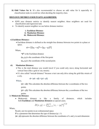
ii. Elbow Method: In the elbow method we plot the model’s error rate or accuracy for different
values of k. As we increase k the error usually decreases initially.
 However after a certain point the error rate starts to decrease more slowly.
 This point where the curve forms an “elbow” that point is considered as best k.
Fig: Elbow Method

35. iii. Odd Values for k: It’s also recommended to choose an odd value for k especially in
classification tasks to avoid ties when deciding the majority class.
DISTANCE METRICS USED IN KNN ALGORITHM:
 KNN uses distance metrics to identify nearest neighbor; these neighbors are used for
classification and regression task.
 To identify nearest neighbor we use below distance metrics:
i. Euclidean Distance
ii. Manhattan Distance
iii. Minkowski Distance
vi.Euclidean Distance:
 Euclidean distance is defined as the straight-line distance between two points in a plane or
space.
Where,
“d” is the Euclidean distance
(x1, y1) is the coordinate of the first point
(x2, y2) is the coordinate of the second point.
vii. Manhattan Distance:
 This is the total distance you would travel if you could only move along horizontal and
vertical lines (like a grid or city streets).
 It’s also called “taxicab distance” because a taxi can only drive along the grid-like streets of
a city.
d = |x1 - x2| + |y1 - y2|
Where,
|x1 - x2|: This calculates the absolute difference between the x-coordinates of the two
points.
|y1 - y2|: This calculates the absolute difference between the y-coordinates of the two
points.
3. Minkowski Distance
 Minkowski distance is like a family of distances, which includes
both Euclidean and Manhattan distances as special cases.
Where,
X and y are two points in an n-dimensional space
P is a parameter that determines the type of distance (p ≥ 1)
|xi - yi| represents the absolute difference between the coordinates of x and y in each dimension

36. Applications of the KNN Algorithm:
 Recommendation Systems
 Spam Detection
 Customer Segmentation
 Speech Recognition
Advantages of the KNN Algorithm:
 Easy to implement
 No training required
 Few Hyper parameters
 Flexible: It works for Classification problem like is this email spam and also work
for Regression task like predicting house prices based on nearby similar houses.
Disadvantages of the KNN Algorithm:
 Doesn’t scale well: KNN is considered as a “lazy” algorithm as it is very slow
especially with large datasets
 Curse of Dimensionality: When the number of features increases KNN struggles to
classify data accurately a problem known as curse of dimensionality.
 Prone to over fitting: As the algorithm is affected due to the curse of dimensionality it
is prone to the problem of over fitting as well.