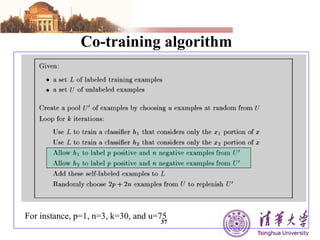
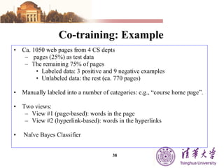
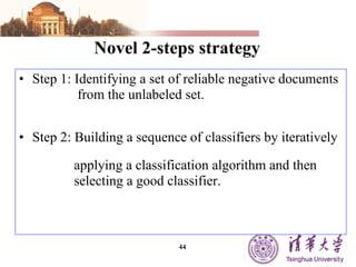
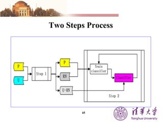
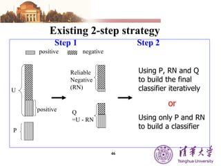
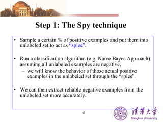
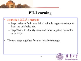
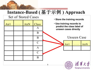
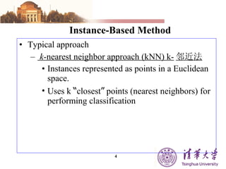
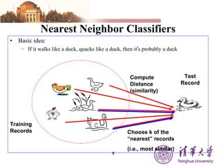
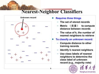
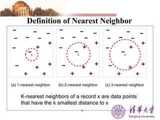
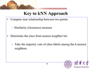
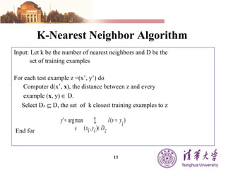
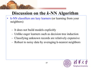
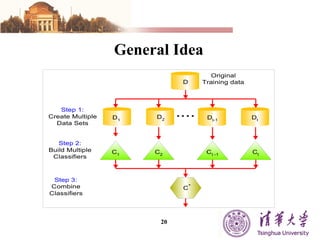
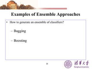
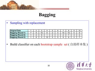
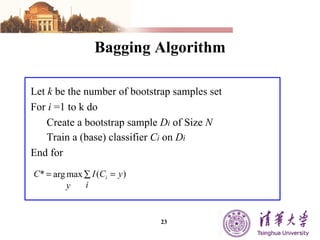
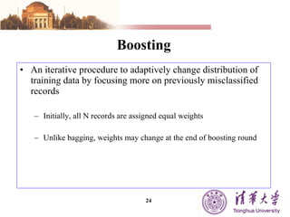
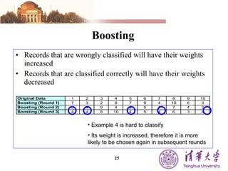
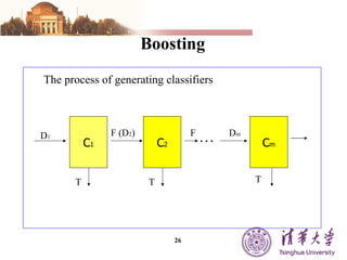
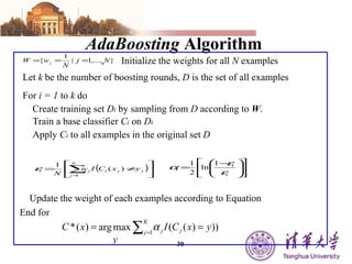
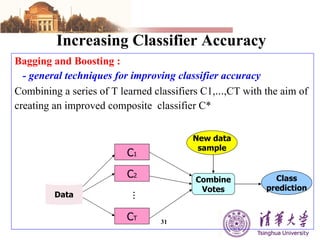
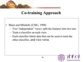
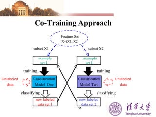
The document summarizes different machine learning classification techniques including instance-based approaches, ensemble approaches, co-training approaches, and partially supervised approaches. It discusses k-nearest neighbor classification and how it works. It also explains bagging, boosting, and AdaBoost ensemble methods. Co-training uses two independent views to label unlabeled data. Partially supervised approaches can build classifiers using only positive and unlabeled data.

1. Chapter 6 (Part II) Alternative Classification Technologies 第六章 ( 第二部分 ) 数据分类技术

2. Chapter 6 (II) Alternative Classification Technologies - Instance ( 示例 ) based Approach - Ensemble ( 组合 ) Approach - Co-training Approach - Partially Supervised Approach

3. Instance-Based ( 基于示例 ) Approach Store the training records Use training records to predict the class label of unseen cases directly

4. Instance-Based Method Typical approach k -nearest neighbor approach (kNN) k- 邻近法 Instances represented as points in a Euclidean space. Uses k “ closest ” points (nearest neighbors) for performing classification

5. Nearest Neighbor Classifiers Basic idea: If it walks like a duck, quacks like a duck, then it ’ s probably a duck Training Records Test Record Compute Distance (similarity) Choose k of the “nearest” records (i.e., most similar)

6. Nearest-Neighbor Classifiers Requires three things The set of stored records Metric （度量） to compute distance between records The value of k, the number of nearest neighbors to retrieve To classify an unknown record: Compute distance to other training records Identify k nearest neighbors Use class labels of nearest neighbors to determine the class label of unknown record (e.g., majority vote)

7. Definition of Nearest Neighbor K-nearest neighbors of a record x are data points that have the k smallest distance to x

8. Key to kNN Approach Compute near relationship between two points - Similarity (closeness) measure Determine the class from nearest neighbor list Take the majority vote of class labels among the k-nearest neighbors

9. Distance- based Similarity Measure Distances are normally used to measure the similarity between two data objects Euclidean distance( 欧几里德距离 ): Properties d(i,j)  0 d(i,i) = 0 d(i,j) = d(j,i) d(i,j)  d(i,k) + d(k,j)

10. Boolean type 布尔型 A contingency table for binary data (state value: 0 or 1) Simple matching coefficient( 简单系数匹配 ) Object i Object j

11. Distance based Measure for Categorical Type( 标称型 ) of Data Categorical type i.e., red, yellow, blue, green for the nominal variable color Method: Simple matching m : # of matches, p : total # of variables

12. Distance based Measure for Mixed Types ( 混合型 ) of Data A object (tuple) may contain all the types mentioned above May use a weighted formula to combine their effects. Given p kinds of the different type variables: if x if = x jf =0 (or missing value) ； otherwise f is boolean ( 布尔 ) or categorical ( 标称 ): d ij (f) = 0 if x if = x jf , or d ij (f) =1 f is interval-valued: use the normalized distance

13. K-Nearest Neighbor Algorithm Input: Let k be the number of nearest neighbors and D be the set of training examples For each test example z =(x’, y’) do Computer d(x’, x ), the distance between z and every example ( x , y)  D. Select D z  D, the set of k closest training examples to z End for

14. Measure for Other Types of Data Textual Data: Vector Space Representation A document is represented as a vector: (W1, W2, … … , Wn) Binary: Wi= 1 if the corresponding term i (often a word) is in the document Wi= 0 if the term i is not in the document TF: (Term Frequency) Wi= tfi tfi is the number of times the term occurred in the document

15. Similarity Measure for Textual Data Distance- based Similarity Measure Problems: high dimension and data sparseness

16. Other Similarity Measure The “ closeness ” between documents is calculated as the correlation between the vectors that represent them, using measures such as the cosine of the angle between these two vectors. Cosine measure ( 余弦计算方法 ) ：

17. Discussion on the k -NN Algorithm k-NN classifiers are lazy learners (or learning from your neighbors) It does not build models explicitly Unlike eager learners such as decision tree induction Classifying unknown records are relatively expensive Robust to noisy data by averaging k-nearest neighbors

18. Chapter 6 (II) Alternative Classification Technologies - Instance ( 示例 )based Approach - Ensemble ( 组合 ) Approach - Co-training Approach - Partially Supervised Approach

19. Ensemble Methods Construct a set of classifiers from the training data Predict class label of previously unseen records by aggregating predictions made by multiple classifiers

20. General Idea

21. Examples of Ensemble Approaches How to generate an ensemble of classifiers? Bagging Boosting

22. Bagging Sampling with replacement Build classifier on each bootstrap sample set ( 自助样本集 )

23. Bagging Algorithm Let k be the number of bootstrap samples set For i =1 to k do Create a bootstrap sample D i of Size N Train a (base) classifier C i on D i End for

24. Boosting An iterative procedure to adaptively change distribution of training data by focusing more on previously misclassified records Initially, all N records are assigned equal weights Unlike bagging, weights may change at the end of boosting round

25. Boosting Records that are wrongly classified will have their weights increased Records that are classified correctly will have their weights decreased Example 4 is hard to classify Its weight is increased, therefore it is more likely to be chosen again in subsequent rounds

26. Boosting C 1 T D 1 F (D 2 ) C 2 T D m … C m T The process of generating classifiers F

27. Boosting Problems: How to update the weights of the training examples? How to combine the predictions made by each base classifier?

28. AdaBoosting Algorithm Given ( x j , y j ) : a set of N training examples ( j=1,…,N ) The error rate of a base classifier C i : where I(p) = 1 if p is true, and 0 otherwise. The importance of a classifier C i :

29. AdaBoosting Algorithm The weight update mechanism (Equation): where is the normalization factor: : the weight for example ( x i , y i ) during the round

30. AdaBoosting Algorithm Let k be the number of boosting rounds, D is the set of all examples Update the weight of each examples according to Equation End for , Initialize the weights for all N examples For i = 1 to k do Create training set D i by sampling from D according to W . Train a base classifier C i on D i Apply C i to all examples in the original set D

31. Increasing Classifier Accuracy Bagging and Boosting : - general techniques for improving classifier accuracy Combining a series of T learned classifiers C1, … ,CT with the aim of creating an improved composite classifier C* Data C 1 C T C 2 … Combine Votes New data sample Class prediction

32. Chapter 6 (II) Alternative Classification Technologies - Instance ( 示例 ) based Approach - Ensemble ( 组合 ) Approach - Co-training Approach - Partially Supervised Approach

33. Unlabeled Data One of the bottlenecks of classification is the labeling of a large set of examples (data records or text documents). Often done manually Time consuming Can we label only a small number of examples and make use of a large number of unlabeled data to classifying?

34. Co-training Approach Blum and Mitchell, (CMU, 1998) Two “independent” views: split the features into two sets. Train a classifier on each view. Each classifier labels data that can be used to train the other classifier , and vice versa

35. Co-Training Approach Feature Set X=(X1, X2) Classification Model One Classification Model Two new labeled data set 1 subset X1 subset X2 training training new labeled data set 2 classifying classifying Unlabeled data Unlabeled data example set L example set L

36. Two views Features can be split into two independence sets(views): The instance space: Each example: A pair of views x 1 , x 2 satisfy view independence just in case: Pr[X 1 =x 1 | X 2 =x 2 , Y=y] = Pr[X 1 =x 1 |Y=y] Pr[X 2 =x 2 | X 1 =x 1 , Y=y] = Pr[X 2 =x 2 |Y=y]

37. Co-training algorithm For instance, p=1, n=3, k=30, and u=75

38. Co-training: Example Ca. 1050 web pages from 4 CS depts pages (25%) as test data The remaining 75% of pages Labeled data: 3 positive and 9 negative examples Unlabeled data: the rest (ca. 770 pages) Manually labeled into a number of categories: e.g., “course home page”. Two views: View #1 (page-based): words in the page View #2 (hyperlink-based): words in the hyperlinks Naïve Bayes Classifier

39. Co-training: Experimental Results begin with 12 labeled web pages (course, etc) provide ca. 1,000 additional unlabeled web pages average error: traditional approach 11.1%; average error: co-training 5.0%

40. Chapter 6 (II) Alternative Classification Technologies - Instance ( 示例 ) based Approach - Ensemble ( 组合 ) Approach - Co-training Approach - Partially Supervised Approach

41. Learning from Positive & Unlabeled Data Positive examples : a set of examples of a class P , Unlabeled set : a set U of unlabeled (or mixed) examples with instances from P and also not from P ( negative examples ). Build a classifier : Build a classifier to classify the examples in U and/or future (test) data. Key feature of the problem : no labeled negative training data. We call this problem, PU-learning .

42. Positive und Unlabeled

43. Direct Marketing Company has database with details of its customer – positive examples, but no information on those who are not their customers, i.e., no negative examples . Want to find people who are similar to their customers for marketing. Buy a database consisting of details of people -- who may be potential customers ?

44. Novel 2-steps strategy Step 1: Identifying a set of reliable negative documents from the unlabeled set. Step 2: Building a sequence of classifiers by iteratively applying a classification algorithm and then selecting a good classifier.

45. Two Steps Process

46. Step 1 Step 2 positive negative Reliable Negative (RN) Q =U - RN U P positive Using P, RN and Q to build the final classifier iteratively or Using only P and RN to build a classifier Existing 2-step strategy

47. Step 1: The Spy technique Sample a certain % of positive examples and put them into unlabeled set to act as “spies”. Run a classification algorithm (e.g. Naïve Bayes Approach) assuming all unlabeled examples are negative, we will know the behavior of those actual positive examples in the unlabeled set through the “spies”. We can then extract reliable negative examples from the unlabeled set more accurately.

48. Step 2: Running a classification algorithm iteratively Running a classification algorithm iteratively iteratively using P, RN and Q until this no document from Q can be classified as negative. RN and Q are updated in each iteration

49. PU-Learning Heuristic ( 启发式 ) methods ： Step 1 tries to find some initial reliable negative examples from the unlabeled set. Step 2 tried to identify more and more negative examples iteratively. The two steps together form an iterative strategy