Downloaded 45 times
![INTRODUCTION
R
R [R Development Core Team, 2012] is a free software
environment for statistical computing and graphics.
It provides a wide variety of statistical and graphical
techniques.
R can be extended easily via packages.
There are around 4000 packages available in the CRAN
package repository 3, as on August 1, 2012.](https://image.slidesharecdn.com/dataminingwithr-140607020734-phpapp02/85/Datamining-with-R-8-320.jpg)
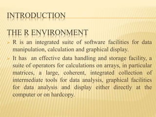
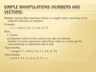
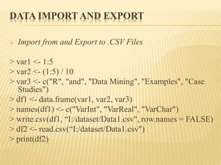
![DATA IMPORT AND EXPORT
Save and Load R Data
Data in R can be saved as .Rdata files with function
save().
> a <- 1:10
> save(a, file=“I:/dataset/Data.Rdata")
> rm(a)
> load(" I:/dataset/Data.Rdata ")
> print(a)
[1] 1 2 3 4 5 6 7 8 9 10](https://image.slidesharecdn.com/dataminingwithr-140607020734-phpapp02/85/Datamining-with-R-19-320.jpg)

The document discusses data mining, defining it as the process of extracting valuable knowledge from large datasets, with primary goals being prediction and description through various tasks such as classification, regression, and clustering. It also introduces R, a statistical computing environment that includes extensive packages for data analysis and manipulation, highlighting features such as command structure and data import/export functionalities. Key R functionalities include vector manipulation, statistical functions, and data management capabilities.


![Introduction to R for Data Science :: Session 6 [Linear Regression in R]](https://cdn.slidesharecdn.com/ss_thumbnails/intrordatasciencesession6eng-160606173046-thumbnail.jpg?width=640&height=640&fit=bounds)