
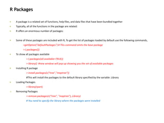
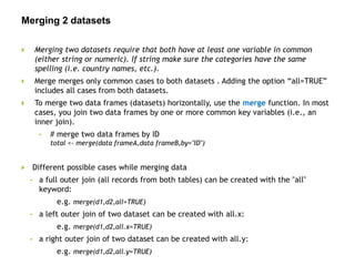
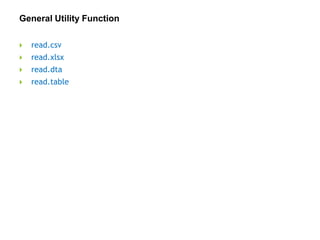
![Basic Operations in R
R has a wide variety of data structures, we will look at few basic ones
Vectors (numerical, character, logical)
Matrices
Data frames
Lists
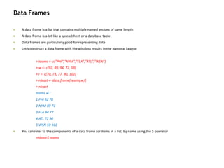
Your first Operations in R
When you enter an expression into the R console and press the Enter key, R will evaluate that expression and display
the results
The interactive R interpreter will automatically print an object returned by an expression entered into the R console
> 1 + 2 + 3
[1] 6
In R, any number that you enter in the console is interpreted as a vector](https://image.slidesharecdn.com/ies-171021112932/85/Big-Data-Mining-in-Indian-Economic-Survey-2017-18-320.jpg)
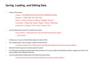
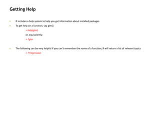
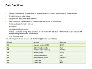
![What is a Vector in R??
A vector is an ordered collection of same data type
The “[1]” means that the index of the first item displayed in the row is 1
You can construct longer vectors using the c(...) function. (c stands for “combine.”)
> c(0, 1, 1, 2, 3, 5, 8)
[1] 0 1 1 2 3 5 8
> 1:50
[1] 1 2 3 4 5 6 7 8 9 10 11 12 13 14 15 16 17 18 19 20 21 22
[23] 23 24 25 26 27 28 29 30 31 32 33 34 35 36 37 38 39 40 41 42 43 44
[45] 45 46 47 48 49 50
The numbers in the brackets on the left hand side of the results indicate the index of the first element shown in each row
When you perform an operation on two vectors, R will match the elements of the two vectors pair wise and return a vector
> c(1, 2, 3, 4) + c(10, 20, 30, 40)
[1] 11 22 33 44
If the two vectors aren’t the same size, R will repeat the smaller sequence multiple times:
> c(1, 2, 3, 4, 5) + c(10, 100)
[1] 11 102 13 104 15
Warning message:
In c(1, 2, 3, 4, 5) + c(10, 100) :
longer object length is not a multiple of shorter object length](https://image.slidesharecdn.com/ies-171021112932/85/Big-Data-Mining-in-Indian-Economic-Survey-2017-20-320.jpg)
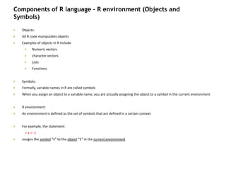
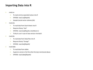
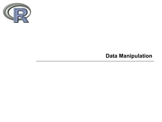
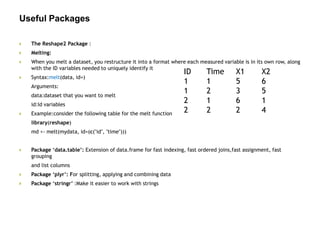
![Arrays
An array is a multidimensional vector.
Vectors and arrays are stored the same way internally, but an array may be displayed differently and accessed differently.
An array object is just a vector that’s associated with a dimension attribute.
Let’s define an array explicitly
>a <- array(c(1,2,3,4,5,6,7,8,9,10,11,12),dim=c(3,4))
> a
[,1] [,2] [,3] [,4]
[1,] 1 4 7 10
[2,] 2 5 8 11
[3,] 3 6 9 12
Here is how you reference one cell
a[2,2]
[1] 5
Arrays can have more than two dimensions.
> w <- array(c(1,2,3,4,5,6,7,8,9,10,11,12,13,14,15,16,17,18),dim=c(3,3,2))
> w](https://image.slidesharecdn.com/ies-171021112932/85/Big-Data-Mining-in-Indian-Economic-Survey-2017-21-320.jpg)
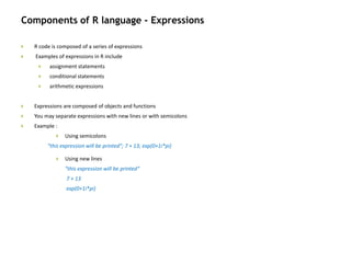
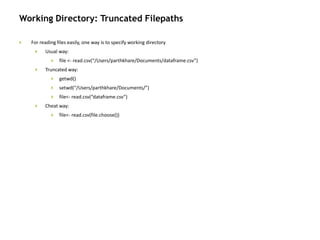
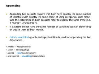
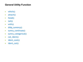
![Arrays & Matrix
R uses very clean syntax for referring to part of an array. You specify separate indices for each dimension, separated by
commas
> w[1,1,1]
[1] 1
To get all rows (or columns) from a dimension, simply omit the indices
> # first row only
> a[1,]
[1] 1 4 7 10
> # first column only
> a[,1]
[1] 1 2 3
A matrix is just a two-dimensional array
> m <- matrix(data=c(1,2,3,4,5,6,7,8,9,10,11,12),nrow=3,ncol=4)
> m
[,1] [,2] [,3] [,4]
[1,] 1 4 7 10
[2,] 2 5 8 11
[3,] 3 6 9 12](https://image.slidesharecdn.com/ies-171021112932/85/Big-Data-Mining-in-Indian-Economic-Survey-2017-22-320.jpg)
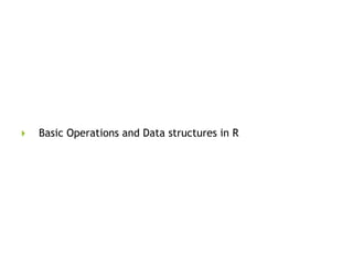
![Lists
It’s possible to construct more complicated structures with multiple data types.
R has a built-in data type for mixing objects of different types, called lists.
Lists in R may contain a heterogeneous selection of objects.
You can name each component in a list.
Items in a list may be referred to by either location or name.
Creating your first list
> e <- list(thing="hat", size="8.25")
> e
You can access an item in the list in multiple ways
Using the name with help of $ operator
> e$thing
Using the location as index
> e[1]
A list can even contain other lists](https://image.slidesharecdn.com/ies-171021112932/85/Big-Data-Mining-in-Indian-Economic-Survey-2017-24-320.jpg)
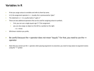
![Revision: Data Structures
Some of the data types are:
• Factor: Categorical variable
• Vector
• Matrix
• Data Frame
• List
To identify the data type of an object we us the function class
> library(datasets)
> air <- airquality
> class(air)
> [1] "data.frame"
Data Types](https://image.slidesharecdn.com/ies-171021112932/85/Big-Data-Mining-in-Indian-Economic-Survey-2017-25-320.jpg)
![Data Types
To check whether the object/variable is of a certain type, use is. functions
is.numeric(), is.character(), is.vector(), is.matrix(), is.data.frame()
These are Logical functions
Returns TRUE/FALSE values
To convert an object/variable of a certain type to another, use as. functions
as.numeric(), as.character(), as.vector(), as.matrix(), as.data.frame(),
as.factor(), as.list()
> is.numeric(airquality$Ozone)
> [1] TRUE
> airquality$Ozone <- as.character(airquality$Ozone)
> is.numeric(airquality$Ozone)
[1] FALSE
> is.character(airquality$Ozone)
> [1] TRUE](https://image.slidesharecdn.com/ies-171021112932/85/Big-Data-Mining-in-Indian-Economic-Survey-2017-26-320.jpg)
![Names, Renaming
Syntax : names(dataset)
> names(airquality)
1] "Ozone" "Solar.R" "Wind" "Temp" "Month" "Day"
> names(airquality) <- NULL
> names(airquality)
> NULL
Renaming
In the following example we will change the variable name “Ozone” to”Oz”
> names(airquality) <- org.names
> names(airquality)[names(airquality)=="Ozone"]= "Oz"
[1] "Oz" "Solar.R" "Wind" "Temp" "Month" "Day"
#Renaming the second variable in data frame “airquality” to “NewName”
> names(airquality)[2] = "Sol"
> names(airquality)
[1] "Oz" "Sol" "Wind" "Temp" "Month" "Day"](https://image.slidesharecdn.com/ies-171021112932/85/Big-Data-Mining-in-Indian-Economic-Survey-2017-33-320.jpg)
![Drop/Keep Variables
Selecting (Keeping) Variables
• # select variables “Ozone “ and “Temp”
> names(airquality) <- org.names
> keep.airquality <- airquality[c("Ozone", “Temp")]
# select 1st and 3rd through 5th variables
> keep.airquality_1 <- airquality[c(1,3:5)]
Excluding (DROPPING) Variables
• Dropping a variable from the dataset can be done by prefixing a “-” sign
before the variable name or the variable index in the Dataframe.
> drop.airquality <- airquality[,c(-3, -4)]](https://image.slidesharecdn.com/ies-171021112932/85/Big-Data-Mining-in-Indian-Economic-Survey-2017-34-320.jpg)
![Subsetting datasets
Subseting is done by using subset function
#subsetting the data set “airquality” where Temperature is greater than 80
> subset_1 <- subset(airquality, Temp>80)
#subsetting the data set “airquality” where Temperature is greater than 80 and finally get only the “Day”
column
> subset_2 = subset(airquality, Temp>80, select=c(“Day"))
#subsetting a column where Temperature is greater than 80 and Day is equal to 8, notice the “==”
> subset_3 = subset(airquality, Temp<80& Day==8)
#subsetting rows without using “subset” function, notice the [ ] square brackets
> subset_4 = airquality[airquality$Temp==80, ]
#We use the %in% notation when we want to subset rows on multiple values of a variable
> subset_5 = airquality[airquality$Temp %in% c(70,90), ]
> subset_5.1 = airquality[airquality$Temp %in% c(70:90), ]](https://image.slidesharecdn.com/ies-171021112932/85/Big-Data-Mining-in-Indian-Economic-Survey-2017-35-320.jpg)
![Sorting
To sort a data frame in R, use the order( ) function. By default, sorting is
ASCENDING. Prepend the sorting variable by a minus sign to indicate
DESCENDING order. Here are some examples.
sorting examples using the mtcars dataset
attach(mtcars)
# sort by hp in ascending order
> sort.mtcars<-mtcars[order(mtcars$hp),]
# sort by hp in discending order
> sort.mtcars<-mtcars[order(-mtcars$hp),]
#Multi level sort a dataset by columns in descending order, put a “-” sign,
> sort.mtcars<-mtcars[order(vs, -mtcars$hp),]](https://image.slidesharecdn.com/ies-171021112932/85/Big-Data-Mining-in-Indian-Economic-Survey-2017-37-320.jpg)
![Remove Duplicate Values
Duplicates are identified using “duplicated” function
#To remove duplicate rows by 2nd column from airquality
> dupair1 = airquality[!duplicated(airquality[,c(2)]),]
#To get duplicate rows in another dataset just remove the “!” sign
> dupair2 = airquality[duplicated(airquality[,c(2)]),]](https://image.slidesharecdn.com/ies-171021112932/85/Big-Data-Mining-in-Indian-Economic-Survey-2017-38-320.jpg)


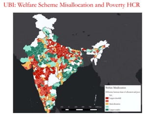
The document provides an introduction to R programming, focusing on its data manipulation capabilities, structures like vectors and data frames, and the functions for importing and exporting data. It discusses topics such as the R environment, basic operations, and the use of packages to enhance functionality. Additionally, it emphasizes the importance of creativity in data analysis, particularly in the context of economic surveys and policy-making.