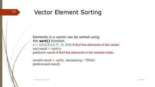
The document provides an introduction to the R programming language, detailing its installation processes for Windows and Linux and basic commands for starting the R interpreter. It covers data types in R, such as vectors, arrays, matrices, and factors, along with examples of how to create and manipulate them. Additionally, it explains how to access and sort vector elements and introduces the concept of factors used for categorizing data.

![Basic Sentence
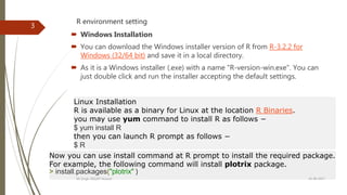
Start your R command prompt by typing the following command (in Linux) −
$ R
OR double click on installed .exe file ( in windows)
This will launch R interpreter and you will get a prompt >
where you can start typing your program as follows −
myString <- "Hello, World!"
> print ( myString)
[1] "Hello, World!"
R Script File
Usually, you will do your programming by writing your programs in script files
and execute those scripts with the help of R interpreter called Rscript. Ex:
# My first program in R Programming
myString <- "Hello, World!“
print ( myString)
Save it as test.R and execute it at R command prompt.
> source(“test.R”)
[1] "Hello, World!"
19-08-2017KK Singh, RGUKT Nuzvid
4](https://image.slidesharecdn.com/2-170819062628/85/2-R-basics-Vectors-Arrays-Matrices-Factors-4-320.jpg)
![Vector-Data Types
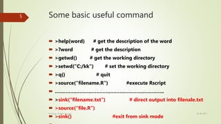
Data Type Example Verify
Logical TRUE, FALSE
v <- TRUE
print(class(v))
[1] "logical"
Numeric 12.3, 5, 999
v <- 23.5
print(class(v))
[1] "numeric"
Integer 2L, 34L, 0L
v <- 2L
print(class(v))
[1] "integer"
Complex 3 + 2i
v <- 2+5i
print(class(v))
[1] "complex"
Character
'a' , '"good",
"TRUE", '23.4'
v <- "TRUE"
print(class(v))
[1] "character" 19-08-2017KK Singh, RGUKT Nuzvid
7](https://image.slidesharecdn.com/2-170819062628/85/2-R-basics-Vectors-Arrays-Matrices-Factors-7-320.jpg)
![Vector (Cont..)
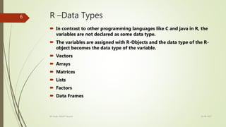
To create vector with more than one element,
use c() function which combines elements into a vector.
# Create a vector.
apple <- c('red','green',"yellow")
print(apple) # Get the class of the vector.
print(class(apple))
………………………………………………………………………..
The non-character values are coerced to character type
if one of the elements is a character.
s <- c('apple','red',5,TRUE)
print(s)
it produces the following result −
[1] "apple" "red" "5" "TRUE"
19-08-2017KK Singh, RGUKT Nuzvid
8](https://image.slidesharecdn.com/2-170819062628/85/2-R-basics-Vectors-Arrays-Matrices-Factors-8-320.jpg)
![Vector (Cont..)
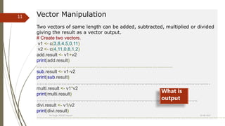
Multiple Elements Vector
Using colon operator with numeric data
# Creating a sequence from 5 to 13.
v <- 5:13
print(v)
……………………………………………………………………………………………
v <- 6.6:12.6 # Creating a sequence from 6.6 to 12.6
print(v)
………………………………………………………………………………………………
# If the final element not belong to the sequence, it is discarded.
v <- 3.8:11.4
print(v)
………………………………………………………………………
Using sequence (Seq.) operator
# Create vector with elements from 5 to 9 incrementing by 0.4.
print(seq(5, 9, by = 0.4))
……………………………………………………………………….
# empty vector
>x<-numeric()
>x[3]<-5
>x
19-08-2017KK Singh, RGUKT Nuzvid
9](https://image.slidesharecdn.com/2-170819062628/85/2-R-basics-Vectors-Arrays-Matrices-Factors-9-320.jpg)
![Accessing vector elements
Accessing Vector Elements
Elements of a Vector are accessed using indexing.
The [ ] brackets are used for indexing. Indexing starts
with position 1.
Giving a negative value in the index drops that element
from result.
TRUE, FALSE or 0 and 1 can also be used for indexing.
# Accessing vector elements using position.
t <- c("Sun","Mon","Tue","Wed","Thurs","Fri","Sat")
u <- t[c(2,3,6)]
print(u)
…………………………………………………………………………………………………….
v <- t[c(TRUE,FALSE,FALSE,FALSE,FALSE,TRUE,FALSE)]
print(v)
……………………………………………………………………………………………………………
……
x <- t[c(-2,-5)] # print t excluding 2nd & 5th index value
print(x)
19-08-2017KK Singh, RGUKT Nuzvid
10](https://image.slidesharecdn.com/2-170819062628/85/2-R-basics-Vectors-Arrays-Matrices-Factors-10-320.jpg)
![Accessing Array Elements# see previous example
print(result[3,,2]) # Print the third row of the second matrix of the array.
print(result[1,3,1]) # Print the element in the 1st row and 3rd column of the 1st matrix.
print(result[,,2]) # Print the 2nd Matrix.
It produces the following result −
COL1 COL2 COL3
3 12 15
[1] 13
COL1 COL2 COL3
ROW1 5 10 13
ROW2 9 11 14
ROW3 3 12 15
Q. Access 2nd & 4th column of the result.
19-08-2017KK Singh, RGUKT Nuzvid
18](https://image.slidesharecdn.com/2-170819062628/85/2-R-basics-Vectors-Arrays-Matrices-Factors-15-320.jpg)
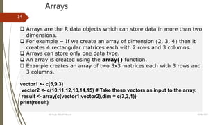
![Manipulating Array Elements
As array is made up matrices in multiple dimensions, the operations
on elements of array are carried out by accessing elements of the matrices.
# Create two vectors of different lengths.
vector1 <- c(5,9,3)
vector2 <- c(10,11,12,13,14,15)
array1 <- array(c(vector1,vector2),dim = c(3,3,2))
vector3 <- c(9,1,0)
vector4 <- c(6,0,11,3,14,1,2,6,9)
array2 <- array(c(vector1,vector2),dim = c(3,3,2))
matrix1 <- array1[,,2]
matrix2 <- array2[,,2]
result <- matrix1+matrix2
print(result)
19-08-2017KK Singh, RGUKT Nuzvid
19](https://image.slidesharecdn.com/2-170819062628/85/2-R-basics-Vectors-Arrays-Matrices-Factors-16-320.jpg)

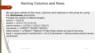
![Accessing Elements of a Matrix
Elements of a matrix can be accessed by using the column and row index of the element.
rownames = c("row1", "row2", "row3", "row4")
colnames = c("col1", "col2", "col3")
P <- matrix(c(3:14), nrow = 4, byrow = TRUE, dimnames = list(rownames, colnames)) # Create the matrix
print(P[1,3]) # Access the element at 3rd column and 1st row.
print(P[4,2]) # Access the element at 2nd column and 4th row.
print(P[2,]) # Access only the 2nd row.
print(P[,3]) # Access only the 3rd column.
It produces the following result −
[1] 5
[1] 13
col1 col2 col3
6 7 8
row1 row2 row3 row4
5 8 11 14
Q. A matrix has 100 columns, access all even index column.
19-08-2017KK Singh, RGUKT Nuzvid
23](https://image.slidesharecdn.com/2-170819062628/85/2-R-basics-Vectors-Arrays-Matrices-Factors-18-320.jpg)
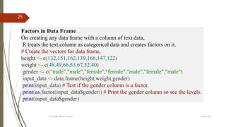
![19-08-2017KK Singh, RGUKT Nuzvid
24
Factorsare the data objects which are used to categorize the data and store it as levels.
They can store both strings and integers.
They are useful in the columns which have a limited number of unique values.
Like "Male, "Female" and True, False etc. They are useful in data analysis for statistical modeling.
Factors are created using the factor () function by taking a vector as input.
Example
# Create a vector as input.
data <- c("East","West","East","North","North","East","West","West","West","East","North")
print(data)
print(is.factor(data)) # Apply the factor function.
factor_data <- as.factor(data)
print(factor_data)
print(is.factor(factor_data))
It produces the following result −
[1] "East" "West" "East" "North" "North" "East" "West" "West" "West" "East" "North"
[1] FALSE
[1] East West East North North East West West West East North Levels: East North West
[1] TRUE](https://image.slidesharecdn.com/2-170819062628/85/2-R-basics-Vectors-Arrays-Matrices-Factors-19-320.jpg)