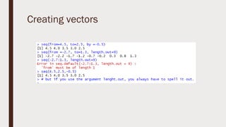
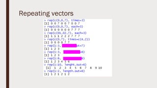
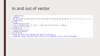
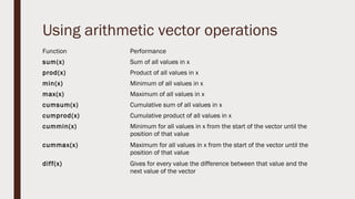
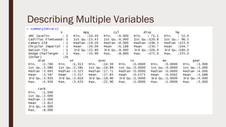
The document provides an overview of R programming, emphasizing its functionality as a statistical processing environment and a tool for data analysis. It covers R Studio's interface components, basic arithmetic operations, and the creation and manipulation of vectors and data frames. Additionally, it discusses data visualization techniques, statistical testing, and model prediction with an emphasis on the importance of splitting datasets for improving predictive accuracy.

1. R

2. R =
programming language,
a statistical processing environment,
a way to solve problems,
and
a collection of helpful tools to make your life easier.

3. RGui desktop Icon
Console based
R prompt >
R Studio is a code editor and development
environment with some very nice features that make
code development easy

4. 1. Source
2.
Console
3. Environment and
History
4. Files, Plots, Packages, Help and
Viewer

5. Source
■ Top left corner of the screen contains a text editor that lets you work with source
script files.
■ Here, you can enter multiple lines of code, save your script files to disk, and perform
other tasks on your script.
■ It recognizes and highlights various elements of your code

6. Console
■ This is where you do all the interactive work with R.

7. Environment and History
■ Here you can inspect the variables you created in your session, as well as their
values.
■ This is also the area where you can see a history of the commands you have issued
in R

8. Files, plots, package, help, and viewer
■ Files: this is where you can browse the folders and files on your computer.
■ Plots: this is where R displays your plots.
■ Packages: You can view a list of all installed packages. A package is a self contained
set of code that adds functionality to R, similar to the way that adds-in add
functionality to MS-Excel.
■ Help: This is where you can browse R’s built in help system.
■ Viewer: This is where R Studio displays previews of some advanced features, such
as dynamic web pages and presentations that you can create with R and add-on
packages.

9. Let’s start with R….

10. By the way, we shall start with
simple program.
Simple math
Sequencing =looks like a colon (:)

11. Vector
■ A vector is the simplest type of data structure in R.
■ Vector = a single entity consisting of a collection of things.
■ For e.g. A collection of numbers, for example, is a numeric vector.

12. Storing and calculating values
= and <- are same

13. Saving work
■ Several options are here:
– You can save individual variables with the save() function
– You can save the entire environment with save.image () function.
– You can save your R script file, using the appropriate save menu command in
your code editor.

14. ■ Find out which working directory R will use to save your file by typing the following
– getwd()
■ Type the following code in your console, using a filename and press entre:
– save(yourname, file=yourname.rda)
■ To make sure that the operation was successful, use your file browser to navigate to
the working directory, and see
– See the lower panel of R-studio

15. Basic Arithmetic
Operator Description Example
x+y y added to x 2+3=5
x-y Y subtracted from x 8-2=6
x*y X multiplied by y 3*2=6
x/y X divided by y 20/10=2
x^y X raised to the power y 3^2=9
x%%y Reminder of x divided by y 7%%3=1
x%/%y X divided by y but rounded down 7%/%3=2

16. Order of operations
■ Exponentiation
■ Multiplication and division in the order in which the operators are presented
■ Addition and subtraction in the order in which the operators are presented
■ The mode operator(%%) and the integer division operator (%/%) have the same
priority as the normal division operator(/) in calculations.
■ Everything that is put in between parentheses is carried out first.

17. Mathematical functions
Function Performance
abs (x) Absolute value of x
log (x, base=y) Logarithm of x with base y, if base in not specified, returns to natural
logarithm
exp(x) Exponential of x
sqrt(x) Square root of x
factorial (x) Factorial of x i.e. x!
choose (x,y) Returns the number of possible combination when drawing y elements at
a time from x possibilities

18. Organizing data in vectors
■ Most powerful feature in R
■ Vector is one-dimensional set of values, all the same type.
■ R use both numeric and strings based data as vector
■ Vectors have a structure and a type, and R is a bit sensitive about both.

20. Creating vectors

21. Repeating vectors

22. In and out of vector

23. Using arithmetic vector operations
Function Performance
sum(x) Sum of all values in x
prod(x) Product of all values in x
min(x) Minimum of all values in x
max(x) Maximum of all values in x
cumsum(x) Cumulative sum of all values in x
cumprod(x) Cumulative product of all values in x
cummin(x) Minimum for all values in x from the start of the vector until the
position of that value
cummax(x) Maximum for all values in x from the start of the vector until the
position of that value
diff(x) Gives for every value the difference between that value and the
next value of the vector

25. Scan ■ Command c() is tedious
■ data=scan()
?

26. Character Command
Scan(what=‘character’)

27. Using the Clipboard to Make
Data
The scan() command is easier to use than the c() command because it does not require
commas. The command can also be used in conjunction with the clipboard, which is
quite useful for entering data from other programs (for example, a spreadsheet). To use
these commands, perform the following steps:
1 . If the data are numbers in a spreadsheet, simply type the command in
R as usual before switching to the spreadsheet containing the data.
2 . Highlight the necessary cells in the spreadsheet and copy them to the
clipboard.
3 . Return to R and paste the data from the clipboard into R. As usual, R
waits until a blank line is entered before ending the data entry so you can continue
to copy and paste more data as required.
4 . Once you are finished, enter a blank line to complete data entry. If the
data are text, you add the what =‘character’ instruction to the scan() command as

28. Before that concept of
Getwd()
Setwd() must be clear

29. Reading bigger data files
■ The scan() command is helpful to read a simple vector.
■ But not useful to read two-dimensional items containing both row and columns.
■ Then we use read.csv() command to take data from spread sheet.

31. Alternative commands
read.table()
read.delim()

32. data.frames
■ Most useful feature of R
■ data.frame is just like an Excel spread sheet in that it has rows and columns.
■ Each columns is a variable and each row is an observation.
■ Each columns is actually a vector with same length
■ Within a column each element must be of the same type, just like with vectors.
■ Numerous way to construct data frames.

37. Home work: Practice various forms of checking Row and columns from text book

38. Manipulating vectors

39. Sorting and rearranging

40. Sorting and rearranging

41. Summary
■ mean(mtcars$mpg)
■ median(mtcars$mpg)
■ sd(mtcars$mpg)
■ range(mtcars$mpg)
■ quantile(mtcars$mpg)

42. Plotting histogram

44. Describing Multiple Variables

48. Summary Stats for Matrix objects

50. Contingency Tables
■ A way of redrawing data and assemble it into a table that shows the layout of the
original data in a manner that allows the reader to gain an overall summary of the
original data.
■ Command table()
■ Command can handle data in simple vectors or more complex matrix and data
frame objects.

52. Task for students:
Creating Custo m Co ntingency Table

53. Summary Command on Contingency Table

56. Data Distribution
■ Histogram we have already done it.

57. Box plots

59. Customization of Boxplots

60. Scatter Plot

61. Customization of Scatter Plot & Pair
Plots

62. Bar Chart
■ Single Category bar chart
■ Multiple category bar chart

63. Simple Hypothesis testing
■ Two sample t-test with unequal variance
■ Two sample t-test with equal variance

64. One sample t-test

65. Directional Hypothesis

66. Excercise
■ File name orchid
■ Available in data frame
■ So use of attach & detach file will be there

68. Paired t-test

69. Correlation

70. Regression for practioners
■ File name CARS
■ Speed and Distance

71. Graphical Analysis
■ Scatter plot: Visualize the linear relationship between the predictor and response
■ Box plot: To spot any outlier observations in the variable. Having outliers in your
predictor can drastically affect the predictions as they can easily affect the
direction/slope of the line of best fit.
■ Density plot: To see the distribution of the predictor variable. Ideally, a close to
normal distribution (a bell shaped curve), without being skewed to the left or right is
preferred. Let us see how to make each one of them.

76. STATISTIC CRITERION
R-Squared Higher the better (> 0.70)
Adj R-Squared Higher the better
F-Statistic Higher the better
Std. Error Closer to zero the better
t-statistic
Should be greater 1.96 for p-value to be
less than 0.05
AIC Lower the better
BIC Lower the better
Mallows cp
Should be close to the number of predictors
in model
MAPE (Mean absolute percentage error) Lower the better
MSE (Mean squared error) Lower the better
Min_Max Accuracy => mean(min(actual,
predicted)/max(actual, predicted))
Higher the better

77. Predicting Linear Model
■ So far we have seen how to build a linear regression model using the whole dataset.
If we build it that way, there is no way to tell how the model will perform with new
data. So the preferred practice is to split your dataset into a 80:20 sample
(training:test), then, build the model on the 80% sample and then use the model
thus built to predict the dependent variable on test data.
■ Doing it this way, we will have the model predicted values for the 20% data (test) as
well as the actuals (from the original dataset). By calculating accuracy measures
(like min_max accuracy) and error rates (MAPE or MSE), we can find out the
prediction accuracy of the model. Now, lets see how to actually do this.

78. Step 1: Create the training
(development) and test (validation) data
samples from original data.

79. Step 2: Develop the model on the
training data and use it to predict the
distance on test data

80. Step 3: Review diagnostic
measures. From the model summary,
the model p value and
predictor’s p value are less
than the significance level,
so we know we have a
statistically significant
model.
Also, the R-Sq and Adj R-Sq
are comparative to the
original model built on full
data.

81. Step 4: Calculate prediction
accuracy and error rates