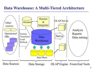
1
Chapter 4: Data Warehousing and On-line
Analytical Processing
 Data Warehouse: Basic Concepts
 Data Warehouse Modeling: Data Cube and OLAP
 Data Warehouse Design and Usage
 Data Warehouse Implementation
 Data Generalization by Attribute-Oriented
Induction
 Summary
2
What is a Data Warehouse?
 “A data warehouse is a subject-oriented, integrated, time-variant,
and nonvolatile collection of data in support of management’s
decision-making process.”—W. H. Inmon
 Data warehousing:
 The process of constructing, maintaining and using data
warehouses
3
Data Warehouse—Subject-Oriented
 Organized around major subjects, such as customer,
product, sales
 Focus is on the modeling and analysis of data for
decision makers, not on daily operations or transaction
processing
 Provide a simple and concise view around particular
subject issues by excluding data that are not useful in
the decision support process
4
Data Warehouse—Integrated
 Constructed by integrating multiple, heterogeneous data
sources
 relational databases, flat files, on-line transaction
records
 Data cleaning and data integration techniques are
applied.
 Ensure consistency in naming conventions, encoding
structures, attribute measures, etc. among different
data sources
 E.g., Hotel price: currency, tax, breakfast covered, etc.
 When data is moved to the warehouse, it is converted
into information.
5
Data Warehouse—Time Variant
 The time horizon for the data warehouse is significantly
longer than that of operational systems
 Operational database: maintains current data
 Data warehouse data: provide information from a
historical perspective (e.g., past 5-10 years)
 Every key structure in the data warehouse
 Contains an element of time, explicitly or implicitly
 But the operational database may or may not involve
“time element”
6
Data Warehouse—Nonvolatile
 A physically separate store of data obtained from the
operational environment
 Operational update of data does not occur in the data
warehouse environment
 Does not require transaction processing, recovery,
and concurrency control mechanisms
 Requires only two operations in data accessing:
 initial loading of data and accessing / reading data
7
OLTP vs. OLAP
OLTP OLAP
users clerk, IT professional knowledge worker
function day to day operations decision support
DB design application-oriented subject-oriented
data current, up-to-date
detailed, flat relational
isolated
historical,
summarized, multidimensional
integrated, consolidated
usage repetitive ad-hoc
access read/write
index/hash on prim. key
lots of scans
unit of work short, simple transaction complex query
# records accessed tens millions
#users thousands hundreds
DB size 100MB-GB 100GB-TB
metric transaction throughput query throughput, response
8
Why a Separate Data Warehouse?
 High performance for both systems
 DBMS— tuned for OLTP: access methods, indexing, concurrency
control, recovery
 Warehouse—tuned for OLAP: complex OLAP queries,
multidimensional view, consolidation of data in the form of
information
 Different functions and different data:
 Current vs historical data: Decision support requires historical data
which operational DBs do not typically maintain
 data consolidation: Decision Support requires consolidation
(aggregation, summarization) of data from heterogeneous sources
 data quality: different sources typically use inconsistent data
representations, codes and formats which have to be reconciled
 Note: It is possible to perform OLAP analysis directly on relational
databases
9
Data Warehouse: A Multi-Tiered Architecture
Data
Warehouse
Extract
Transform
Load
Refresh
OLAP Engine
Analysis
Reports
Data mining
Monitor
&
Integrator
Metadata
Data Sources Front-End Tools
Serve
Data Marts
Operational
DBs
Other
sources
Data Storage
OLAP Server
10
Three Data Warehouse Models
 Enterprise warehouse
 collects all the information about various subjects
spanning the entire organization
 Data Mart
 a subset of corporate-wide data that is of value to a
specific groups of users. Its scope is confined to
specific, selected groups, such as marketing data mart
 Independent vs. dependent (directly from warehouse) data marts
 Virtual warehouse
 A set of views over operational databases are created
 Very limited number of the possible summary views may
be materialized
11
Extraction, Transformation, and Loading (ETL)
 Data extraction
 get data from multiple, heterogeneous, and external
sources
 Data cleaning
 detect errors in the data and rectify them when possible
 Data transformation
 convert data from legacy or host format to warehouse
format
 Load
 sort, summarize, consolidate, compute views, and build
indicies and partitions
 Refresh
 propagate the updates from the data sources to the
warehouse periodically
12
Metadata Repository
 Meta data is the data defining warehouse objects. It stores:
 Description of the structure of the data warehouse
 schema, view, dimensions, hierarchies, derived data defn, data
mart locations and contents
 Operational meta-data
 data lineage (history of migrated data and transformation path),
timing of data (active, or archived,), monitoring information
(warehouse usage statistics, error reports, audit trails)
 The algorithms used for summarization
 The mapping from operational environment to the data warehouse
 Data related to system performance
 Business data
 business terms and definitions, ownership of data, charging policies
13
Chapter 4: Data Warehousing and On-line
Analytical Processing
 Data Warehouse: Basic Concepts
 Data Warehouse Modeling: Data Cube and OLAP
 Data Warehouse Design and Usage
 Data Warehouse Implementation
 Data Generalization by Attribute-Oriented
Induction
 Summary
14
From Tables and Spreadsheets to
Data Cubes
 A data warehouse is based on a multidimensional data model in order to
view the data at various levels of granularity in the form of a data cube
 A data cube for a subject, such as sales, allows data to be modeled and
viewed in multiple dimensions. It contains
 Dimension tables, such as item (item_name, brand, type), or
time(day, week, month, quarter, year)
 Fact table contains measures (such as units_sold) for different
contexts composed of keys to each of the related dimension table entries
 In an n-D data cube, an n-D fact table is modeled as the base cuboid and its
further summarization over selected subset of dimensions provide lower-
dimensional cuboids arranged in a lattice. The ultimate summarization over
all dimensions results in 0-D cuboid, which is called apex cuboid.
15
Cube: A Lattice of Cuboids
time,item
time,item,location
time, item, location, supplier
all
time item location supplier
time,location
time,supplier
item,location
item,supplier
location,supplier
time,item,supplier
time,location,supplier
item,location,supplier
0-D (apex) cuboid
1-D cuboids
2-D cuboids
3-D cuboids
4-D (base) cuboid
16
Conceptual Modeling of Data Warehouses
 Modeling data warehouses: dimensions & measures
 Star schema: A fact table in the middle connected to a
set of dimension tables
 Snowflake schema: A refinement of star schema
where some dimensional hierarchy is normalized into a
set of smaller dimension tables, forming a shape
similar to snowflake
 Fact constellations: Multiple fact tables share
dimension tables, viewed as a collection of stars,
therefore called galaxy schema or fact constellation
17
Example of Star Schema
time_key
day
day_of_the_week
month
quarter
year
time
location_key
street
city
state_or_province
country
location
Sales Fact Table
time_key
item_key
branch_key
location_key
units_sold
sale_amount
avg_sales
Measures
item_key
item_name
brand
type
supplier_type
item
branch_key
branch_name
branch_type
branch
18
Example of Snowflake Schema
time_key
day
day_of_the_week
month
quarter
year
time
location_key
street
city_key
location
Sales Fact Table
time_key
item_key
branch_key
location_key
units_sold
sale_amount
avg_sales
Measures
item_key
item_name
brand
type
supplier_key
item
branch_key
branch_name
branch_type
branch
supplier_key
supplier_type
supplier
city_key
city
state_or_province
country
city
19
Example of Fact Constellation
time_key
day
day_of_the_week
month
quarter
year
time
location_key
street
city
province_or_state
country
location
Sales Fact Table
time_key
item_key
branch_key
location_key
units_sold
sale_amount
avg_sales
Measures
item_key
item_name
brand
type
supplier_type
item
branch_key
branch_name
branch_type
branch
Shipping Fact Table
time_key
item_key
shipper_key
from_location
to_location
dollars_cost
units_shipped
shipper_key
shipper_name
location_key
shipper_type
shipper
20
Data Cube Measures: Three Categories
 Distributive: if the result derived by applying the function
to n partial aggregate values is the same as that derived
by applying the function on all the data without partitioning
 E.g., count(), sum(), min(), max()
 Algebraic: if it can be computed by an algebraic function
with M arguments (where M is a bounded integer), each of
which is obtained by applying a distributive aggregate
function
 E.g., avg(), min_N(), standard_deviation()
 Holistic: if there is no algebraic function to compute the
measure in terms of multiple subaggregates derived for
data partitions. E.g., median(), mode(), rank()
21
A Concept Hierarchy:
Dimension (location)
all
Europe Asia
China
India
Spain
Germany
Vizag
MVP
Peda Waltair
...
...
...
... ...
...
all
region
locality
country
Hyderabad
Frankfurt
city
22
Multidimensional Data
 Sales volume as a function of product, month,
and region
Product
Month
Dimensions: Product, Location, Time
Hierarchical summarization paths
Industry Region Year
Category Country Quarter
Product City Month Week
Office Day
23
A Sample Data Cube
Total annual sales
of TVs in U.S.A.
Date
Country
sum
sum
TV
VCR
PC
1Qtr 2Qtr 3Qtr 4Qtr
U.S.A
Canada
Mexico
sum
Cuboids presented in the Data Cube
February 15, 2024 Data Mining: Concepts and Techniques 24
25
Typical OLAP Operations
 Roll up (drill-up): summarize data
 by climbing up hierarchy or by dimension reduction
 Drill down (roll down): reverse of roll-up
 from higher level summary to lower level summary or
detailed data, or introducing new dimensions
 Slice and dice: project and select
 Pivot (rotate):
 reorient the cube, visualization, 3D to series of 2D planes
 Other operations
 drill across: involving (across) more than one fact table
 drill through: through the bottom level of the cube to its
back-end relational tables (using SQL)
26
Fig. 3.10 Typical OLAP
Operations
27
Chapter 4: Data Warehousing and On-line
Analytical Processing
 Data Warehouse: Basic Concepts
 Data Warehouse Modeling: Data Cube and OLAP
 Data Warehouse Design and Usage
 Data Warehouse Implementation
 Data Generalization by Attribute-Oriented
Induction
 Summary
28
Data Warehouse Development:
A Recommended Approach
Define a high-level corporate data model
Data
Mart
Data
Mart
Distributed
Data Marts
Multi-Tier Data
Warehouse
Enterprise
Data
Warehouse
Model refinement
Model refinement
29
Data Warehouse Usage
 Three kinds of data warehouse applications
 Information processing
 supports querying, basic statistical analysis, and reporting
using crosstabs, tables, charts and graphs
 Analytical processing
 multidimensional analysis of data warehouse data
 supports basic OLAP operations, slice-dice, drilling, pivoting
 Data mining
 knowledge discovery from hidden patterns
 supports associations, constructing analytical models,
performing classification and prediction, and presenting the
mining results using visualization tools
30
Chapter 4: Data Warehousing and On-line
Analytical Processing
 Data Warehouse: Basic Concepts
 Data Warehouse Modeling: Data Cube and OLAP
 Data Warehouse Design and Usage
 Data Warehouse Implementation
 Data Generalization by Attribute-Oriented
Induction
 Summary
31
Efficient Data Cube Computation
 Data cube can be viewed as a lattice of cuboids
 The bottom-most cuboid is the base cuboid
 The top-most cuboid (apex) contains only one cell
 How many cuboids constitute an n-dimensional cube
with Li levels for i-th dimension?
 Each dimension can be represented at any of the possible Li +1 levels
(+1 for total collapsing)
 Materialization of data cube
 Materialize every (cuboid) (full materialization),
none (no materialization), or some (partial
materialization)
 Selection of which cuboids to materialize
 Based on size, sharing, access frequency, etc.
)
1
1
( 



n
i
i
L
T
32
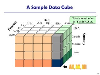
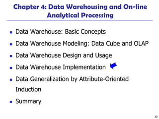
The “Compute Cube” Operator
 Cube definition and computation in DMQL
define cube sales [item, city, year]: sum (sale amount)
compute cube sales
 Transform it into a SQL-like language (with a new operator cube by)
SELECT item, city, year, SUM (sale amount)
FROM SALES
CUBE BY item, city, year
 Need to compute following Group-Bys
( item, city, year),
(item,year),(city,year), (city,item),
(year), (item), (city)
()
(item)
(city)
()
(year)
(city, item) (city, year) (item, year)
(city, item, year)
33
Indexing OLAP Data: Bitmap Index
 Bit map index is an alternative representation of record Id list.
 Each attribute value pair has a distinct bit vector and hence an attribute
having v distinct values has a bitmap index containing v bit vectors
 The length of each bit vector is equal to # of records in the base table
 The i-th bit is set if the i-th row of the base table has the value same as
that of the indexed column
 Since bit-wise operations are fast, bitmap index reduces access time, and
since the strings are represented by single bits, space and I/O reduces
 But, it is not suitable for high cardinality attributes
Cust Region Type
C1 Asia Retail
C2 Europe Dealer
C3 Asia Dealer
C4 America Retail
C5 Europe Dealer
RecID Retail Dealer
1 1 0
2 0 1
3 0 1
4 1 0
5 0 1
RecID Asia Europe America
1 1 0 0
2 0 1 0
3 1 0 0
4 0 0 1
5 0 1 0
Base table Index on Region Index on Type
34
Indexing OLAP Data: Join Indices
 Join index registers the joinable rows of two
relations from a Relational DB
 Join index: JI(R-id, S-id) is created where R
(R-id, A)  S (S-id, B) are joinable on A and
B
 It materializes relational join in JI file to
speed up relational join
 In data warehouses, join index relates the
values of the dimensions of a star schema to
rows in the fact table.
E.g. Sales fact table and two dimensions city
and product
A join index on city maintains for each
distinct city a list of R-IDs of the fact table
records containing the Sales in the city
Join indices can span over multiple
dimensions
35
Efficiently Processing OLAP Queries
 Determine which operations should be performed on the available cuboids
 Transform selection, projection, drill, roll, etc. required for query answering
into corresponding SQL and/or OLAP operations, e.g., dice = selection +
projection
 Determine which materialized cuboid(s) should be selected for OLAP op.
 Let the query to be processed be on {brand, province_or_state} with the
condition “year = 2022”, and there are 4 materialized cuboids available:
1) {year, item_name, city}
2) {year, brand, country}
3) {year, brand, province_or_state}
4) {item_name, province_or_state} where year = 2022
Which should be selected to process the query?
36
OLAP Server Architectures
 Relational OLAP (ROLAP)
 Use relational or extended-relational DBMS to store and manage
warehouse data and OLAP middle ware
 Include optimization of DBMS backend, implementation of
aggregation navigation logic, and additional tools and services
 Greater scalability
 Multidimensional OLAP (MOLAP)
 Sparse array-based multidimensional storage engine
 Fast indexing to pre-computed summarized data
 Hybrid OLAP (HOLAP) (e.g., Microsoft SQLServer)
 Flexibility, e.g., low level: ROLAP, high-level: MOLAP
 Specialized SQL servers (e.g., Redbricks)
 Specialized support for SQL queries over star/snowflake schemas
37
Chapter 4: Data Warehousing and On-line
Analytical Processing
 Data Warehouse: Basic Concepts
 Data Warehouse Modeling: Data Cube and OLAP
 Data Warehouse Design and Usage
 Data Warehouse Implementation
 Data Generalization by Attribute-Oriented
Induction
 Summary
38
Attribute-Oriented Induction
 How it is done?
 Collect the task-relevant data (initial relation) using a
relational database query
 Perform generalization by attribute removal or
attribute generalization
 Apply aggregation by merging identical, generalized
tuples and accumulating their respective counts
 Interaction with users for knowledge presentation
39
Attribute-Oriented Induction: An Example
Example: Describe general characteristics of graduate
students in the University database
 Step 1. Fetch relevant set of data using an SQL
statement, e.g.,
Select * (i.e., name, gender, major, birth_place,
birth_date, residence, phone#, gpa)
from student
where student_status in {“MSc”, “MCA”, “B.Tech” }
 Step 2. Perform attribute-oriented induction
 Step 3. Present results in generalized relation, cross-tab,
or rule forms
40
Class Characterization: An Example
Name Gender Major Birth-Place Birth_date Residence Phone # GPA
Jim
Woodman
M CS Vancouver,BC,
Canada
8-12-76 3511 Main St.,
Richmond
687-4598 3.67
Scott
Lachance
M CS Montreal, Que,
Canada
28-7-75 345 1st Ave.,
Richmond
253-9106 3.70
Laura Lee
…
F
…
Physics
…
Seattle, WA, USA
…
25-8-70
…
125 Austin Ave.,
Burnaby
…
420-5232
…
3.83
…
Removed Retained Sci,Eng,
Bus
Country Age range City Removed Excl,
VG,..
Gender Major Birth_region Age_range Residence GPA Count
M Science Canada 20-25 Richmond Very-good 16
F Science Foreign 25-30 Burnaby Excellent 22
… … … … … … …
Birth_Region
Gender
Canada Foreign Total
M 16 14 30
F 10 22 32
Total 26 36 62
Prime
Generalized
Relation
Initial
Relation
41
Basic Principles of Attribute-Oriented Induction
 Data focusing: task-relevant data, including dimensions,
and the result is the initial relation
 Attribute-generalization: If there is a large set of distinct
values for A, and there exists a set of generalization
operators on A, then select an operator and generalize A
 Attribute-removal: remove attribute A if there is a large set
of distinct values for A but (1) there is no generalization
operator on A, or (2) A’s higher level concepts are
expressed in terms of other attributes
 Attribute-threshold control: typical 2-8, specified/default
 Generalized relation threshold control: control the final
relation/rule size
42
Attribute-Oriented Induction: Basic
Algorithm
 InitialRel: Query processing of task-relevant data to derive
the initial relation.
 PreGen: Based on the analysis of the number of distinct
values in each attribute, determine generalization plan for
each attribute: removal? or how high to generalize?
 PrimeGen: Based on the PreGen plan, perform
generalization to the right level to derive a “prime
generalized relation”, accumulating the counts.
 Presentation: User interaction: (1) adjust levels by drilling,
(2) pivoting, (3) mapping into rules, cross tabs,
visualization presentations.
43
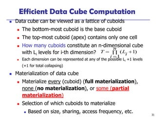
Presentation of Generalized Results
 Generalized relation:
 Relations where some of the attributes are generalized, with counts
or other aggregation values accumulated.
 Cross tabulation:
 Mapping results into cross tabulation form (similar to contingency
tables).
 Visualization techniques:
 Pie charts, bar charts, curves, cubes, and other visual forms.
 Quantitative characteristic rules:
 Mapping generalized result into characteristic rules with quantitative
information associated with it, e.g.,
.
%]
47
:
[
"
"
)
(
_
%]
53
:
[
"
"
)
(
_
)
(
)
(
t
foreign
x
region
birth
t
Canada
x
region
birth
x
male
x
grad





44
Mining Class Comparisons
 Comparison: Comparing two or more classes
 Method:
 Partition the set of relevant data into the target class and the contrasting
class(es)
 Generalize both classes to the same high level concepts
 Compare tuples with the same high level descriptions
 Present for every tuple its description and two measures
 Support or typicality (t-weight) - distribution within single class
 Discrimination (d-weight)- comparing distribution between classes
 Highlight the tuples with strong discriminant features
 Relevance Analysis:
 Find attributes (features) which can distinguish different classes the
most
45
Concept Description vs. Cube-Based OLAP
 Similarity: Both the methods support
 data generalization
 data summarization at multiple levels of abstraction
 interactive drilling, pivoting, slicing and dicing
 Differences:
 OLAP has systematic preprocessing, query independent
summarization, and can drill down on a focused subset to
rather low level
 AOI has automated desired level allocation, and may
perform dimension relevance analysis/ranking when there
are many relevant dimensions
46
Chapter 4: Data Warehousing and On-line
Analytical Processing
 Data Warehouse: Basic Concepts
 Data Warehouse Modeling: Data Cube and OLAP
 Data Warehouse Design and Usage
 Data Warehouse Implementation
 Data Generalization by Attribute-Oriented
Induction
 Summary
47
Summary
 Data warehousing: A multi-dimensional model of a data warehouse
 A data cube consists of dimensions & measures
 Star schema, snowflake schema, fact constellations
 OLAP operations: drilling, rolling, slicing, dicing and pivoting
 Data Warehouse Architecture, Design, and Usage
 Multi-tiered architecture
 Business analysis design framework
 Information processing, analytical processing, data mining
 Implementation: Efficient computation of data cubes
 Partial vs. full vs. no materialization
 Indexing OLAP data: Bitmap index and join index
 OLAP query processing
 OLAP servers: ROLAP, MOLAP, HOLAP
 Data generalization: Attribute-oriented induction

data warehousing and online analtytical processing

  • 1.
    1 Chapter 4: DataWarehousing and On-line Analytical Processing  Data Warehouse: Basic Concepts  Data Warehouse Modeling: Data Cube and OLAP  Data Warehouse Design and Usage  Data Warehouse Implementation  Data Generalization by Attribute-Oriented Induction  Summary
  • 2.
    2 What is aData Warehouse?  “A data warehouse is a subject-oriented, integrated, time-variant, and nonvolatile collection of data in support of management’s decision-making process.”—W. H. Inmon  Data warehousing:  The process of constructing, maintaining and using data warehouses
  • 3.
    3 Data Warehouse—Subject-Oriented  Organizedaround major subjects, such as customer, product, sales  Focus is on the modeling and analysis of data for decision makers, not on daily operations or transaction processing  Provide a simple and concise view around particular subject issues by excluding data that are not useful in the decision support process
  • 4.
    4 Data Warehouse—Integrated  Constructedby integrating multiple, heterogeneous data sources  relational databases, flat files, on-line transaction records  Data cleaning and data integration techniques are applied.  Ensure consistency in naming conventions, encoding structures, attribute measures, etc. among different data sources  E.g., Hotel price: currency, tax, breakfast covered, etc.  When data is moved to the warehouse, it is converted into information.
  • 5.
    5 Data Warehouse—Time Variant The time horizon for the data warehouse is significantly longer than that of operational systems  Operational database: maintains current data  Data warehouse data: provide information from a historical perspective (e.g., past 5-10 years)  Every key structure in the data warehouse  Contains an element of time, explicitly or implicitly  But the operational database may or may not involve “time element”
  • 6.
    6 Data Warehouse—Nonvolatile  Aphysically separate store of data obtained from the operational environment  Operational update of data does not occur in the data warehouse environment  Does not require transaction processing, recovery, and concurrency control mechanisms  Requires only two operations in data accessing:  initial loading of data and accessing / reading data
  • 7.
    7 OLTP vs. OLAP OLTPOLAP users clerk, IT professional knowledge worker function day to day operations decision support DB design application-oriented subject-oriented data current, up-to-date detailed, flat relational isolated historical, summarized, multidimensional integrated, consolidated usage repetitive ad-hoc access read/write index/hash on prim. key lots of scans unit of work short, simple transaction complex query # records accessed tens millions #users thousands hundreds DB size 100MB-GB 100GB-TB metric transaction throughput query throughput, response
  • 8.
    8 Why a SeparateData Warehouse?  High performance for both systems  DBMS— tuned for OLTP: access methods, indexing, concurrency control, recovery  Warehouse—tuned for OLAP: complex OLAP queries, multidimensional view, consolidation of data in the form of information  Different functions and different data:  Current vs historical data: Decision support requires historical data which operational DBs do not typically maintain  data consolidation: Decision Support requires consolidation (aggregation, summarization) of data from heterogeneous sources  data quality: different sources typically use inconsistent data representations, codes and formats which have to be reconciled  Note: It is possible to perform OLAP analysis directly on relational databases
  • 9.
    9 Data Warehouse: AMulti-Tiered Architecture Data Warehouse Extract Transform Load Refresh OLAP Engine Analysis Reports Data mining Monitor & Integrator Metadata Data Sources Front-End Tools Serve Data Marts Operational DBs Other sources Data Storage OLAP Server
  • 10.
    10 Three Data WarehouseModels  Enterprise warehouse  collects all the information about various subjects spanning the entire organization  Data Mart  a subset of corporate-wide data that is of value to a specific groups of users. Its scope is confined to specific, selected groups, such as marketing data mart  Independent vs. dependent (directly from warehouse) data marts  Virtual warehouse  A set of views over operational databases are created  Very limited number of the possible summary views may be materialized
  • 11.
    11 Extraction, Transformation, andLoading (ETL)  Data extraction  get data from multiple, heterogeneous, and external sources  Data cleaning  detect errors in the data and rectify them when possible  Data transformation  convert data from legacy or host format to warehouse format  Load  sort, summarize, consolidate, compute views, and build indicies and partitions  Refresh  propagate the updates from the data sources to the warehouse periodically
  • 12.
    12 Metadata Repository  Metadata is the data defining warehouse objects. It stores:  Description of the structure of the data warehouse  schema, view, dimensions, hierarchies, derived data defn, data mart locations and contents  Operational meta-data  data lineage (history of migrated data and transformation path), timing of data (active, or archived,), monitoring information (warehouse usage statistics, error reports, audit trails)  The algorithms used for summarization  The mapping from operational environment to the data warehouse  Data related to system performance  Business data  business terms and definitions, ownership of data, charging policies
  • 13.
    13 Chapter 4: DataWarehousing and On-line Analytical Processing  Data Warehouse: Basic Concepts  Data Warehouse Modeling: Data Cube and OLAP  Data Warehouse Design and Usage  Data Warehouse Implementation  Data Generalization by Attribute-Oriented Induction  Summary
  • 14.
    14 From Tables andSpreadsheets to Data Cubes  A data warehouse is based on a multidimensional data model in order to view the data at various levels of granularity in the form of a data cube  A data cube for a subject, such as sales, allows data to be modeled and viewed in multiple dimensions. It contains  Dimension tables, such as item (item_name, brand, type), or time(day, week, month, quarter, year)  Fact table contains measures (such as units_sold) for different contexts composed of keys to each of the related dimension table entries  In an n-D data cube, an n-D fact table is modeled as the base cuboid and its further summarization over selected subset of dimensions provide lower- dimensional cuboids arranged in a lattice. The ultimate summarization over all dimensions results in 0-D cuboid, which is called apex cuboid.
  • 15.
    15 Cube: A Latticeof Cuboids time,item time,item,location time, item, location, supplier all time item location supplier time,location time,supplier item,location item,supplier location,supplier time,item,supplier time,location,supplier item,location,supplier 0-D (apex) cuboid 1-D cuboids 2-D cuboids 3-D cuboids 4-D (base) cuboid
  • 16.
    16 Conceptual Modeling ofData Warehouses  Modeling data warehouses: dimensions & measures  Star schema: A fact table in the middle connected to a set of dimension tables  Snowflake schema: A refinement of star schema where some dimensional hierarchy is normalized into a set of smaller dimension tables, forming a shape similar to snowflake  Fact constellations: Multiple fact tables share dimension tables, viewed as a collection of stars, therefore called galaxy schema or fact constellation
  • 17.
    17 Example of StarSchema time_key day day_of_the_week month quarter year time location_key street city state_or_province country location Sales Fact Table time_key item_key branch_key location_key units_sold sale_amount avg_sales Measures item_key item_name brand type supplier_type item branch_key branch_name branch_type branch
  • 18.
    18 Example of SnowflakeSchema time_key day day_of_the_week month quarter year time location_key street city_key location Sales Fact Table time_key item_key branch_key location_key units_sold sale_amount avg_sales Measures item_key item_name brand type supplier_key item branch_key branch_name branch_type branch supplier_key supplier_type supplier city_key city state_or_province country city
  • 19.
    19 Example of FactConstellation time_key day day_of_the_week month quarter year time location_key street city province_or_state country location Sales Fact Table time_key item_key branch_key location_key units_sold sale_amount avg_sales Measures item_key item_name brand type supplier_type item branch_key branch_name branch_type branch Shipping Fact Table time_key item_key shipper_key from_location to_location dollars_cost units_shipped shipper_key shipper_name location_key shipper_type shipper
  • 20.
    20 Data Cube Measures:Three Categories  Distributive: if the result derived by applying the function to n partial aggregate values is the same as that derived by applying the function on all the data without partitioning  E.g., count(), sum(), min(), max()  Algebraic: if it can be computed by an algebraic function with M arguments (where M is a bounded integer), each of which is obtained by applying a distributive aggregate function  E.g., avg(), min_N(), standard_deviation()  Holistic: if there is no algebraic function to compute the measure in terms of multiple subaggregates derived for data partitions. E.g., median(), mode(), rank()
  • 21.
    21 A Concept Hierarchy: Dimension(location) all Europe Asia China India Spain Germany Vizag MVP Peda Waltair ... ... ... ... ... ... all region locality country Hyderabad Frankfurt city
  • 22.
    22 Multidimensional Data  Salesvolume as a function of product, month, and region Product Month Dimensions: Product, Location, Time Hierarchical summarization paths Industry Region Year Category Country Quarter Product City Month Week Office Day
  • 23.
    23 A Sample DataCube Total annual sales of TVs in U.S.A. Date Country sum sum TV VCR PC 1Qtr 2Qtr 3Qtr 4Qtr U.S.A Canada Mexico sum
  • 24.
    Cuboids presented inthe Data Cube February 15, 2024 Data Mining: Concepts and Techniques 24
  • 25.
    25 Typical OLAP Operations Roll up (drill-up): summarize data  by climbing up hierarchy or by dimension reduction  Drill down (roll down): reverse of roll-up  from higher level summary to lower level summary or detailed data, or introducing new dimensions  Slice and dice: project and select  Pivot (rotate):  reorient the cube, visualization, 3D to series of 2D planes  Other operations  drill across: involving (across) more than one fact table  drill through: through the bottom level of the cube to its back-end relational tables (using SQL)
  • 26.
    26 Fig. 3.10 TypicalOLAP Operations
  • 27.
    27 Chapter 4: DataWarehousing and On-line Analytical Processing  Data Warehouse: Basic Concepts  Data Warehouse Modeling: Data Cube and OLAP  Data Warehouse Design and Usage  Data Warehouse Implementation  Data Generalization by Attribute-Oriented Induction  Summary
  • 28.
    28 Data Warehouse Development: ARecommended Approach Define a high-level corporate data model Data Mart Data Mart Distributed Data Marts Multi-Tier Data Warehouse Enterprise Data Warehouse Model refinement Model refinement
  • 29.
    29 Data Warehouse Usage Three kinds of data warehouse applications  Information processing  supports querying, basic statistical analysis, and reporting using crosstabs, tables, charts and graphs  Analytical processing  multidimensional analysis of data warehouse data  supports basic OLAP operations, slice-dice, drilling, pivoting  Data mining  knowledge discovery from hidden patterns  supports associations, constructing analytical models, performing classification and prediction, and presenting the mining results using visualization tools
  • 30.
    30 Chapter 4: DataWarehousing and On-line Analytical Processing  Data Warehouse: Basic Concepts  Data Warehouse Modeling: Data Cube and OLAP  Data Warehouse Design and Usage  Data Warehouse Implementation  Data Generalization by Attribute-Oriented Induction  Summary
  • 31.
    31 Efficient Data CubeComputation  Data cube can be viewed as a lattice of cuboids  The bottom-most cuboid is the base cuboid  The top-most cuboid (apex) contains only one cell  How many cuboids constitute an n-dimensional cube with Li levels for i-th dimension?  Each dimension can be represented at any of the possible Li +1 levels (+1 for total collapsing)  Materialization of data cube  Materialize every (cuboid) (full materialization), none (no materialization), or some (partial materialization)  Selection of which cuboids to materialize  Based on size, sharing, access frequency, etc. ) 1 1 (     n i i L T
  • 32.
    32 The “Compute Cube”Operator  Cube definition and computation in DMQL define cube sales [item, city, year]: sum (sale amount) compute cube sales  Transform it into a SQL-like language (with a new operator cube by) SELECT item, city, year, SUM (sale amount) FROM SALES CUBE BY item, city, year  Need to compute following Group-Bys ( item, city, year), (item,year),(city,year), (city,item), (year), (item), (city) () (item) (city) () (year) (city, item) (city, year) (item, year) (city, item, year)
  • 33.
    33 Indexing OLAP Data:Bitmap Index  Bit map index is an alternative representation of record Id list.  Each attribute value pair has a distinct bit vector and hence an attribute having v distinct values has a bitmap index containing v bit vectors  The length of each bit vector is equal to # of records in the base table  The i-th bit is set if the i-th row of the base table has the value same as that of the indexed column  Since bit-wise operations are fast, bitmap index reduces access time, and since the strings are represented by single bits, space and I/O reduces  But, it is not suitable for high cardinality attributes Cust Region Type C1 Asia Retail C2 Europe Dealer C3 Asia Dealer C4 America Retail C5 Europe Dealer RecID Retail Dealer 1 1 0 2 0 1 3 0 1 4 1 0 5 0 1 RecID Asia Europe America 1 1 0 0 2 0 1 0 3 1 0 0 4 0 0 1 5 0 1 0 Base table Index on Region Index on Type
  • 34.
    34 Indexing OLAP Data:Join Indices  Join index registers the joinable rows of two relations from a Relational DB  Join index: JI(R-id, S-id) is created where R (R-id, A)  S (S-id, B) are joinable on A and B  It materializes relational join in JI file to speed up relational join  In data warehouses, join index relates the values of the dimensions of a star schema to rows in the fact table. E.g. Sales fact table and two dimensions city and product A join index on city maintains for each distinct city a list of R-IDs of the fact table records containing the Sales in the city Join indices can span over multiple dimensions
  • 35.
    35 Efficiently Processing OLAPQueries  Determine which operations should be performed on the available cuboids  Transform selection, projection, drill, roll, etc. required for query answering into corresponding SQL and/or OLAP operations, e.g., dice = selection + projection  Determine which materialized cuboid(s) should be selected for OLAP op.  Let the query to be processed be on {brand, province_or_state} with the condition “year = 2022”, and there are 4 materialized cuboids available: 1) {year, item_name, city} 2) {year, brand, country} 3) {year, brand, province_or_state} 4) {item_name, province_or_state} where year = 2022 Which should be selected to process the query?
  • 36.
    36 OLAP Server Architectures Relational OLAP (ROLAP)  Use relational or extended-relational DBMS to store and manage warehouse data and OLAP middle ware  Include optimization of DBMS backend, implementation of aggregation navigation logic, and additional tools and services  Greater scalability  Multidimensional OLAP (MOLAP)  Sparse array-based multidimensional storage engine  Fast indexing to pre-computed summarized data  Hybrid OLAP (HOLAP) (e.g., Microsoft SQLServer)  Flexibility, e.g., low level: ROLAP, high-level: MOLAP  Specialized SQL servers (e.g., Redbricks)  Specialized support for SQL queries over star/snowflake schemas
  • 37.
    37 Chapter 4: DataWarehousing and On-line Analytical Processing  Data Warehouse: Basic Concepts  Data Warehouse Modeling: Data Cube and OLAP  Data Warehouse Design and Usage  Data Warehouse Implementation  Data Generalization by Attribute-Oriented Induction  Summary
  • 38.
    38 Attribute-Oriented Induction  Howit is done?  Collect the task-relevant data (initial relation) using a relational database query  Perform generalization by attribute removal or attribute generalization  Apply aggregation by merging identical, generalized tuples and accumulating their respective counts  Interaction with users for knowledge presentation
  • 39.
    39 Attribute-Oriented Induction: AnExample Example: Describe general characteristics of graduate students in the University database  Step 1. Fetch relevant set of data using an SQL statement, e.g., Select * (i.e., name, gender, major, birth_place, birth_date, residence, phone#, gpa) from student where student_status in {“MSc”, “MCA”, “B.Tech” }  Step 2. Perform attribute-oriented induction  Step 3. Present results in generalized relation, cross-tab, or rule forms
  • 40.
    40 Class Characterization: AnExample Name Gender Major Birth-Place Birth_date Residence Phone # GPA Jim Woodman M CS Vancouver,BC, Canada 8-12-76 3511 Main St., Richmond 687-4598 3.67 Scott Lachance M CS Montreal, Que, Canada 28-7-75 345 1st Ave., Richmond 253-9106 3.70 Laura Lee … F … Physics … Seattle, WA, USA … 25-8-70 … 125 Austin Ave., Burnaby … 420-5232 … 3.83 … Removed Retained Sci,Eng, Bus Country Age range City Removed Excl, VG,.. Gender Major Birth_region Age_range Residence GPA Count M Science Canada 20-25 Richmond Very-good 16 F Science Foreign 25-30 Burnaby Excellent 22 … … … … … … … Birth_Region Gender Canada Foreign Total M 16 14 30 F 10 22 32 Total 26 36 62 Prime Generalized Relation Initial Relation
  • 41.
    41 Basic Principles ofAttribute-Oriented Induction  Data focusing: task-relevant data, including dimensions, and the result is the initial relation  Attribute-generalization: If there is a large set of distinct values for A, and there exists a set of generalization operators on A, then select an operator and generalize A  Attribute-removal: remove attribute A if there is a large set of distinct values for A but (1) there is no generalization operator on A, or (2) A’s higher level concepts are expressed in terms of other attributes  Attribute-threshold control: typical 2-8, specified/default  Generalized relation threshold control: control the final relation/rule size
  • 42.
    42 Attribute-Oriented Induction: Basic Algorithm InitialRel: Query processing of task-relevant data to derive the initial relation.  PreGen: Based on the analysis of the number of distinct values in each attribute, determine generalization plan for each attribute: removal? or how high to generalize?  PrimeGen: Based on the PreGen plan, perform generalization to the right level to derive a “prime generalized relation”, accumulating the counts.  Presentation: User interaction: (1) adjust levels by drilling, (2) pivoting, (3) mapping into rules, cross tabs, visualization presentations.
  • 43.
    43 Presentation of GeneralizedResults  Generalized relation:  Relations where some of the attributes are generalized, with counts or other aggregation values accumulated.  Cross tabulation:  Mapping results into cross tabulation form (similar to contingency tables).  Visualization techniques:  Pie charts, bar charts, curves, cubes, and other visual forms.  Quantitative characteristic rules:  Mapping generalized result into characteristic rules with quantitative information associated with it, e.g., . %] 47 : [ " " ) ( _ %] 53 : [ " " ) ( _ ) ( ) ( t foreign x region birth t Canada x region birth x male x grad     
  • 44.
    44 Mining Class Comparisons Comparison: Comparing two or more classes  Method:  Partition the set of relevant data into the target class and the contrasting class(es)  Generalize both classes to the same high level concepts  Compare tuples with the same high level descriptions  Present for every tuple its description and two measures  Support or typicality (t-weight) - distribution within single class  Discrimination (d-weight)- comparing distribution between classes  Highlight the tuples with strong discriminant features  Relevance Analysis:  Find attributes (features) which can distinguish different classes the most
  • 45.
    45 Concept Description vs.Cube-Based OLAP  Similarity: Both the methods support  data generalization  data summarization at multiple levels of abstraction  interactive drilling, pivoting, slicing and dicing  Differences:  OLAP has systematic preprocessing, query independent summarization, and can drill down on a focused subset to rather low level  AOI has automated desired level allocation, and may perform dimension relevance analysis/ranking when there are many relevant dimensions
  • 46.
    46 Chapter 4: DataWarehousing and On-line Analytical Processing  Data Warehouse: Basic Concepts  Data Warehouse Modeling: Data Cube and OLAP  Data Warehouse Design and Usage  Data Warehouse Implementation  Data Generalization by Attribute-Oriented Induction  Summary
  • 47.
    47 Summary  Data warehousing:A multi-dimensional model of a data warehouse  A data cube consists of dimensions & measures  Star schema, snowflake schema, fact constellations  OLAP operations: drilling, rolling, slicing, dicing and pivoting  Data Warehouse Architecture, Design, and Usage  Multi-tiered architecture  Business analysis design framework  Information processing, analytical processing, data mining  Implementation: Efficient computation of data cubes  Partial vs. full vs. no materialization  Indexing OLAP data: Bitmap index and join index  OLAP query processing  OLAP servers: ROLAP, MOLAP, HOLAP  Data generalization: Attribute-oriented induction