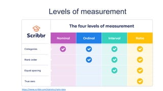
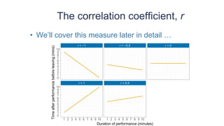
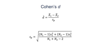
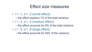
Learning Module 1
Course Preparation:
Basic Statistical Concepts
Types of data analysis
• Quantitative Methods
– Testing theories using numbers
• Qualitative Methods
– Testing theories using language
• Magazine articles/Interviews
• Conversations
• Newspapers
• Media broadcasts
The research process
Test your theory
• Hypothesis:
– Coca-cola kills sperm.
• Independent Variable
– The proposed cause
– A predictor variable
– A manipulated variable (in experiments)
– Coca-cola in the hypothesis above
• Dependent Variable
– The proposed effect
– An outcome variable
– Measured not manipulated (in experiments)
– Sperm in the hypothesis above
Levels of measurement
• Categorical (entities are divided into distinct categories):
– Binary variable: There are only two categories
• e.g. dead or alive.
– Nominal variable: There are more than two categories
• e.g. whether someone is an omnivore, vegetarian, vegan, or fruitarian.
– Ordinal variable: The same as a nominal variable but the categories have a
logical order
• e.g. whether people got a fail, a pass, a merit or a distinction in their exam.
• Continuous (entities get a distinct score):
– Interval variable: Equal intervals on the variable represent equal differences in
the property being measured
• e.g. the difference between 6 and 8 is equivalent to the difference between 13 and 15.
– Ratio variable: The same as an interval variable, but the ratios of scores on the
scale must also make sense
• e.g. a score of 16 on an anxiety scale means that the person is, in reality, twice as anxious
as someone scoring 8.
https://www.scribbr.com/statistics/ratio-data
Validity
• Whether an instrument measures what it set out to
measure.
• Content validity
– Evidence that the content of a test corresponds to the
content of the construct it was designed to cover
• Ecological validity
– Evidence that the results of a study, experiment or test
can be applied, and allow inferences, to real-world
conditions.
Reliability
• Reliability
– The ability of the measure to produce the same results
under the same conditions.
• Test-Retest Reliability
– The ability of a measure to produce consistent results
when the same entities are tested at two different points
in time.
How to measure
• Correlational research:
– Observing what naturally goes on in the world without
directly interfering with it.
• Experimental research:
– One or more variable is systematically manipulated to
see their effect (alone or in combination) on an outcome
variable.
– Statements can be made about cause and effect.
Types of variation
• Systematic Variation
– Differences in performance created by a specific
experimental manipulation.
• Unsystematic Variation
– Differences in performance created by unknown factors.
• Age, Gender, IQ, Time of day, Measurement error etc.
• Randomization
– Minimizes unsystematic variation.
Analysing data: histograms
• Frequency Distributions (aka Histograms)
– A graph plotting values of observations on the horizontal
axis, with a bar showing how many times each value
occurred in the data set.
• The ‘Normal’ Distribution
– Bell shaped
– Symmetrical around the centre
The normal distribution
The curve shows the idealized shape.
0
1000
2000
3000
−4 −2 0 2 4
Score
Frequency
Properties of frequency distributions
• Skew
– The symmetry of the distribution.
– Positive skew (scores bunched at low values with the tail
pointing to high values).
– Negative skew (scores bunched at high values with the tail
pointing to low values).
• Kurtosis
– The ‘heaviness’ of the tails.
– Leptokurtic = heavy tails.
– Platykurtic = light tails.
Skew
Positive skew Negative skew
0
1000
2000
3000
4000
Frequency
Kurtosis
Leptokurtic Platykurtic
0
3000
6000
9000
Frequency
Central tendency: the mode
• Mode
– The most frequent score
• Bimodal
– Having two modes
• Multimodal
– Having several modes
Central tendency: the median
• The Median is the middle score when scores are
ordered:
Central tendency: the mean
• Mean
– The sum of scores divided by the number
of scores.
– Number of friends of 11 Facebook users.
The dispersion: range
• The Range
– The smallest score subtracted from the largest
– For our Facebook friends data the highest score is 234
and the lowest is 22; therefore the range is: 234 −22 =
212
The dispersion: the interquartile range
• Quartiles
– The three values that split the sorted data into four
equal parts.
– Second Quartile = median.
– Lower quartile = median of lower half of the data
– Upper quartile = median of upper half of the data
Sum of squared errors, SS
• Indicates the total dispersion, or total deviance of scores
from the mean:
• More useful to work with the average dispersion, known as
the variance:
Standard deviation
• The variance gives us a measure in units squared.
– In our Facebook example we would have to say
that the average error in out data was 3224.6
friends squared.
• This problem is solved by taking the square root of
the variance, which is known as the standard
deviation:
Important things to remember
• The sum of squares, variance, and standard
deviation represent the same thing:
– The ‘Fit’ of the mean to the data
– The variability in the data
– How well the mean represents the observed data
– Error
Going beyond the data: z-scores
• Z-scores
– Standardising a score with respect to the other
scores in the group.
– Expresses a score in terms of how many
standard deviations it is away from the mean.
– The distribution of z-scores has a mean of 0
and SD = 1.
s
X
X
z
−
=
Probability density function of a normal
distribution
z
Density
0.00
0.05
0.10
0.15
0.20
0.25
0.30
0.35
0.40
●
●
●
●
●
●
●
●
●
●
●
●
●
●
●
●
●
●
●
●
●
●
●
●
●
●
●
●
●
●
●
●
●
●
●
●
●
●
●
●
●
●
●
●
●
●
●
●
●
●
●
●
●
●
●
●
●
●
●
●
●
●
●
●
●
●
●
●
●
●
●
●
●
●
●
●
●
●
●
●
●
●
●
●
●
●
●
●
●
●
●
●
●
●
●
●
●
●
●
●
●
●
●
●
●
●
●
●
●
●
●
●
●
●
●
●
●
●
●
●
●
●
●
●
●
●
●
●
●
●
●
●
●
●
●
●
●
●
●
●
●
●
●
●
●
●
●
●
●
●
●
●
●
●
●
●
●
●
●
●
●
●
●
●
●
●
●
●
●
●
●
●
●
●
●
●
●
●
●
●
●
●
●
●
●
●
●
●
●
●
●
●
●
●
●
●
●
●
●
●
●
●
●
●
●
●
●
●
●
●
●
●
●
●
●
●
●
●
●
●
●
●
●
●
●
●
●
●
●
●
●
●
●
●
●
●
●
●
●
●
●
●
●
●
●
●
●
●
●
●
●
●
●
●
●
●
●
●
●
●
●
●
●
●
●
●
●
●
●
●
●
●
●
●
●
●
●
●
●
●
●
●
●
●
●
●
●
●
●
●
●
●
●
●
●
●
●
●
●
●
●
●
●
●
●
●
●
●
●
●
●
●
●
●
●
●
●
●
●
●
●
●
●
●
●
●
●
●
●
●
●
●
●
●
●
●
●
●
●
●
●
●
●
●
●
●
●
●
●
●
●
●
●
●
●
●
●
●
●
●
●
●
●
●
●
●
●
●
●
●
●
●
●
●
●
●
●
●
●
●
●
●
●
●
●
●
●
●
●
●
●
●
●
●
●
●
●
●
●
●
●
●
●
●
●
●
●
●
●
●
●
●
●
●
●
●
●
●
●
●
●
●
●
●
●
●
●
●
●
●
●
●
●
●
●
●
●
●
●
●
●
●
●
●
●
●
●
●
●
●
●
●
●
●
●
●
●
●
●
●
●
●
●
●
●
●
●
●
●
●
●
●
●
●
●
●
●
●
●
●
●
●
●
●
●
●
●
●
●
●
●
●
●
●
●
●
●
●
●
●
●
●
●
●
●
●
●
●
●
●
●
●
●
●
●
●
●
●
●
●
●
●
●
●
●
●
●
●
●
●
●
●
●
●
●
●
●
●
●
●
●
●
●
●
●
●
●
●
●
●
●
●
●
●
●
●
●
●
●
●
●
●
●
●
●
●
●
●
●
●
●
●
●
●
●
●
●
●
●
●
●
●
●
●
●
●
●
●
●
●
●
●
●
●
●
●
●
●
●
●
●
●
●
●
●
●
●
●
●
●
●
●
●
●
●
●
●
●
●
●
●
●
●
●
●
●
●
●
●
●
●
●
●
●
●
●
●
●
●
●
●
●
●
●
●
●
●
●
●
●
●
●
●
●
●
●
●
●
●
●
●
●
●
●
●
●
●
●
●
●
●
●
●
●
●
●
●
●
●
●
●
●
●
●
●
●
●
●
●
●
●
●
●
●
●
●
●
●
●
●
●
●
●
●
●
●
●
●
●
●
●
●
●
●
●
●
●
●
●
●
●
●
●
●
●
●
●
●
●
●
●
●
●
●
●
●
●
●
●
●
●
●
●
●
●
●
●
●
●
●
●
●
●
●
●
●
●
●
●
●
●
●
●
●
●
●
●
●
●
●
●
●
●
●
●
●
●
●
●
●
●
●
●
●
●
●
●
●
●
●
●
●
●
●
●
●
●
●
●
●
●
−4.00 −3.00 −1.96 −1.00 0.00 1.00 1.65 1.96 3.00 4.00
Probability = .025 Probability = .025
Probability = .95
Populations and samples
• Population
– The collection of units (be they people, plankton, plants,
cities, suicidal authors, etc.) to which we want to
generalize a set of findings or a statistical model.
• Sample
– A smaller (but hopefully representative) collection of units
from a population used to determine truths about that
population
Samples and populations
• Sample
– Mean and Standard Deviation(SD) describe only the sample from
which they were calculated.
• Population
– Mean and SD are intended to describe the entire population (very
rare in Psychology).
• Sample to population:
– Mean and SD are obtained from a sample, but are used to estimate
the mean and SD of the population (very common in psychology).
N
s
X
=

0
1
2
3
1 2 3 4 5
Sample mean
Frequency
Population
µ = 3
M = 3
Mean = 3 SD = 1.22
True value
(parameter)
Estimates
(statistics)
M = 3
M = 3
M = 4
M = 4
M = 2
M = 2
M= 5
M = 1
Standard Error
Types of hypotheses
• Null hypothesis, H0
• There is no effect.
• E.g. Big Brother contestants and members of the public will not differ in
their scores on personality disorder questionnaires
• The alternative hypothesis, H1
• AKA the experimental hypothesis
• E.g. Big Brother contestants will score higher on personality disorder
questionnaires than members of the public
Type I and Type II errors
• Type I error
– Occurs when we believe that there is a genuine effect in
our population, when in fact there isn’t.
– The probability is the α-level (usually 0.05)
• Type II error
– Occurs when we believe that there is no effect in the
population when, in reality, there is.
– The probability is the β-level (often 0.2)
Misconceptions around p-values
• Misconception 1: A significant result means that the
effect is important
– No, because significance depends on sample size.
• Misconception 2: A non-significant result means that the
null hypothesis is true
– No, a non-significant result tells us only that the effect is not
big enough to be found (given our sample size), it doesn’t tell
us that the effect size is zero.
• Misconception 3: A significant result means that the null
hypothesis is false?
– No, it is logically not possible to conclude this .
Effect sizes
• An effect size is a standardized measure of the size
of an effect:
– Standardized = comparable across studies
– Not (as) reliant on the sample size
– Allows people to objectively evaluate the size of observed
effect.
Effect size measures
• There are several effect size measures that can be
used:
– Cohen’s d
– Pearson’s r
The correlation coefficient, r
• We’ll cover this measure later in detail …
r = −1 r = −0.5 r = 0
r = 1 r = 0.5
0
1
2
3
4
5
6
7
8
9
10
0
1
2
3
4
5
6
7
8
9
10
1 2 3 4 5 6 7 8 9 10 1 2 3 4 5 6 7 8 9 10
Duration of performance (minutes)
Time
after
performance
before
leaving
(mins)
Cohen’s d
መ
𝑑 =
ത
𝑋1 − ത
𝑋2
𝑠𝑝
𝑠𝑝 =
𝑁1 − 1 𝑠1
2
+ 𝑁2 − 1 𝑠2
2
𝑁1 + 𝑁2 − 2
Effect size measures
• r = .1, d = .2 (small effect):
– the effect explains 1% of the total variance.
• r = .3, d = .5 (medium effect):
– the effect accounts for 9% of the total variance.
• r = .5, d = .8 (large effect):
– the effect accounts for 25% of the variance.

Basic Statistical Concepts.pdf

  • 1.
    Learning Module 1 CoursePreparation: Basic Statistical Concepts
  • 2.
    Types of dataanalysis • Quantitative Methods – Testing theories using numbers • Qualitative Methods – Testing theories using language • Magazine articles/Interviews • Conversations • Newspapers • Media broadcasts
  • 3.
  • 4.
    Test your theory •Hypothesis: – Coca-cola kills sperm. • Independent Variable – The proposed cause – A predictor variable – A manipulated variable (in experiments) – Coca-cola in the hypothesis above • Dependent Variable – The proposed effect – An outcome variable – Measured not manipulated (in experiments) – Sperm in the hypothesis above
  • 5.
    Levels of measurement •Categorical (entities are divided into distinct categories): – Binary variable: There are only two categories • e.g. dead or alive. – Nominal variable: There are more than two categories • e.g. whether someone is an omnivore, vegetarian, vegan, or fruitarian. – Ordinal variable: The same as a nominal variable but the categories have a logical order • e.g. whether people got a fail, a pass, a merit or a distinction in their exam. • Continuous (entities get a distinct score): – Interval variable: Equal intervals on the variable represent equal differences in the property being measured • e.g. the difference between 6 and 8 is equivalent to the difference between 13 and 15. – Ratio variable: The same as an interval variable, but the ratios of scores on the scale must also make sense • e.g. a score of 16 on an anxiety scale means that the person is, in reality, twice as anxious as someone scoring 8. https://www.scribbr.com/statistics/ratio-data
  • 6.
    Validity • Whether aninstrument measures what it set out to measure. • Content validity – Evidence that the content of a test corresponds to the content of the construct it was designed to cover • Ecological validity – Evidence that the results of a study, experiment or test can be applied, and allow inferences, to real-world conditions.
  • 7.
    Reliability • Reliability – Theability of the measure to produce the same results under the same conditions. • Test-Retest Reliability – The ability of a measure to produce consistent results when the same entities are tested at two different points in time.
  • 8.
    How to measure •Correlational research: – Observing what naturally goes on in the world without directly interfering with it. • Experimental research: – One or more variable is systematically manipulated to see their effect (alone or in combination) on an outcome variable. – Statements can be made about cause and effect.
  • 9.
    Types of variation •Systematic Variation – Differences in performance created by a specific experimental manipulation. • Unsystematic Variation – Differences in performance created by unknown factors. • Age, Gender, IQ, Time of day, Measurement error etc. • Randomization – Minimizes unsystematic variation.
  • 10.
    Analysing data: histograms •Frequency Distributions (aka Histograms) – A graph plotting values of observations on the horizontal axis, with a bar showing how many times each value occurred in the data set. • The ‘Normal’ Distribution – Bell shaped – Symmetrical around the centre
  • 11.
    The normal distribution Thecurve shows the idealized shape. 0 1000 2000 3000 −4 −2 0 2 4 Score Frequency
  • 12.
    Properties of frequencydistributions • Skew – The symmetry of the distribution. – Positive skew (scores bunched at low values with the tail pointing to high values). – Negative skew (scores bunched at high values with the tail pointing to low values). • Kurtosis – The ‘heaviness’ of the tails. – Leptokurtic = heavy tails. – Platykurtic = light tails.
  • 13.
    Skew Positive skew Negativeskew 0 1000 2000 3000 4000 Frequency
  • 14.
  • 15.
    Central tendency: themode • Mode – The most frequent score • Bimodal – Having two modes • Multimodal – Having several modes
  • 16.
    Central tendency: themedian • The Median is the middle score when scores are ordered:
  • 17.
    Central tendency: themean • Mean – The sum of scores divided by the number of scores. – Number of friends of 11 Facebook users.
  • 18.
    The dispersion: range •The Range – The smallest score subtracted from the largest – For our Facebook friends data the highest score is 234 and the lowest is 22; therefore the range is: 234 −22 = 212
  • 19.
    The dispersion: theinterquartile range • Quartiles – The three values that split the sorted data into four equal parts. – Second Quartile = median. – Lower quartile = median of lower half of the data – Upper quartile = median of upper half of the data
  • 20.
    Sum of squarederrors, SS • Indicates the total dispersion, or total deviance of scores from the mean: • More useful to work with the average dispersion, known as the variance:
  • 21.
    Standard deviation • Thevariance gives us a measure in units squared. – In our Facebook example we would have to say that the average error in out data was 3224.6 friends squared. • This problem is solved by taking the square root of the variance, which is known as the standard deviation:
  • 22.
    Important things toremember • The sum of squares, variance, and standard deviation represent the same thing: – The ‘Fit’ of the mean to the data – The variability in the data – How well the mean represents the observed data – Error
  • 23.
    Going beyond thedata: z-scores • Z-scores – Standardising a score with respect to the other scores in the group. – Expresses a score in terms of how many standard deviations it is away from the mean. – The distribution of z-scores has a mean of 0 and SD = 1. s X X z − =
  • 24.
    Probability density functionof a normal distribution z Density 0.00 0.05 0.10 0.15 0.20 0.25 0.30 0.35 0.40 ● ● ● ● ● ● ● ● ● ● ● ● ● ● ● ● ● ● ● ● ● ● ● ● ● ● ● ● ● ● ● ● ● ● ● ● ● ● ● ● ● ● ● ● ● ● ● ● ● ● ● ● ● ● ● ● ● ● ● ● ● ● ● ● ● ● ● ● ● ● ● ● ● ● ● ● ● ● ● ● ● ● ● ● ● ● ● ● ● ● ● ● ● ● ● ● ● ● ● ● ● ● ● ● ● ● ● ● ● ● ● ● ● ● ● ● ● ● ● ● ● ● ● ● ● ● ● ● ● ● ● ● ● ● ● ● ● ● ● ● ● ● ● ● ● ● ● ● ● ● ● ● ● ● ● ● ● ● ● ● ● ● ● ● ● ● ● ● ● ● ● ● ● ● ● ● ● ● ● ● ● ● ● ● ● ● ● ● ● ● ● ● ● ● ● ● ● ● ● ● ● ● ● ● ● ● ● ● ● ● ● ● ● ● ● ● ● ● ● ● ● ● ● ● ● ● ● ● ● ● ● ● ● ● ● ● ● ● ● ● ● ● ● ● ● ● ● ● ● ● ● ● ● ● ● ● ● ● ● ● ● ● ● ● ● ● ● ● ● ● ● ● ● ● ● ● ● ● ● ● ● ● ● ● ● ● ● ● ● ● ● ● ● ● ● ● ● ● ● ● ● ● ● ● ● ● ● ● ● ● ● ● ● ● ● ● ● ● ● ● ● ● ● ● ● ● ● ● ● ● ● ● ● ● ● ● ● ● ● ● ● ● ● ● ● ● ● ● ● ● ● ● ● ● ● ● ● ● ● ● ● ● ● ● ● ● ● ● ● ● ● ● ● ● ● ● ● ● ● ● ● ● ● ● ● ● ● ● ● ● ● ● ● ● ● ● ● ● ● ● ● ● ● ● ● ● ● ● ● ● ● ● ● ● ● ● ● ● ● ● ● ● ● ● ● ● ● ● ● ● ● ● ● ● ● ● ● ● ● ● ● ● ● ● ● ● ● ● ● ● ● ● ● ● ● ● ● ● ● ● ● ● ● ● ● ● ● ● ● ● ● ● ● ● ● ● ● ● ● ● ● ● ● ● ● ● ● ● ● ● ● ● ● ● ● ● ● ● ● ● ● ● ● ● ● ● ● ● ● ● ● ● ● ● ● ● ● ● ● ● ● ● ● ● ● ● ● ● ● ● ● ● ● ● ● ● ● ● ● ● ● ● ● ● ● ● ● ● ● ● ● ● ● ● ● ● ● ● ● ● ● ● ● ● ● ● ● ● ● ● ● ● ● ● ● ● ● ● ● ● ● ● ● ● ● ● ● ● ● ● ● ● ● ● ● ● ● ● ● ● ● ● ● ● ● ● ● ● ● ● ● ● ● ● ● ● ● ● ● ● ● ● ● ● ● ● ● ● ● ● ● ● ● ● ● ● ● ● ● ● ● ● ● ● ● ● ● ● ● ● ● ● ● ● ● ● ● ● ● ● ● ● ● ● ● ● ● ● ● ● ● ● ● ● ● ● ● ● ● ● ● ● ● ● ● ● ● ● ● ● ● ● ● ● ● ● ● ● ● ● ● ● ● ● ● ● ● ● ● ● ● ● ● ● ● ● ● ● ● ● ● ● ● ● ● ● ● ● ● ● ● ● ● ● ● ● ● ● ● ● ● ● ● ● ● ● ● ● ● ● ● ● ● ● ● ● ● ● ● ● ● ● ● ● ● ● ● ● ● ● ● ● ● ● ● ● ● ● ● ● ● ● ● ● ● ● ● ● ● ● ● ● ● ● ● ● ● ● ● ● ● −4.00 −3.00 −1.96 −1.00 0.00 1.00 1.65 1.96 3.00 4.00 Probability = .025 Probability = .025 Probability = .95
  • 25.
    Populations and samples •Population – The collection of units (be they people, plankton, plants, cities, suicidal authors, etc.) to which we want to generalize a set of findings or a statistical model. • Sample – A smaller (but hopefully representative) collection of units from a population used to determine truths about that population
  • 26.
    Samples and populations •Sample – Mean and Standard Deviation(SD) describe only the sample from which they were calculated. • Population – Mean and SD are intended to describe the entire population (very rare in Psychology). • Sample to population: – Mean and SD are obtained from a sample, but are used to estimate the mean and SD of the population (very common in psychology).
  • 27.
    N s X =  0 1 2 3 1 2 34 5 Sample mean Frequency Population µ = 3 M = 3 Mean = 3 SD = 1.22 True value (parameter) Estimates (statistics) M = 3 M = 3 M = 4 M = 4 M = 2 M = 2 M= 5 M = 1 Standard Error
  • 28.
    Types of hypotheses •Null hypothesis, H0 • There is no effect. • E.g. Big Brother contestants and members of the public will not differ in their scores on personality disorder questionnaires • The alternative hypothesis, H1 • AKA the experimental hypothesis • E.g. Big Brother contestants will score higher on personality disorder questionnaires than members of the public
  • 30.
    Type I andType II errors • Type I error – Occurs when we believe that there is a genuine effect in our population, when in fact there isn’t. – The probability is the α-level (usually 0.05) • Type II error – Occurs when we believe that there is no effect in the population when, in reality, there is. – The probability is the β-level (often 0.2)
  • 31.
    Misconceptions around p-values •Misconception 1: A significant result means that the effect is important – No, because significance depends on sample size. • Misconception 2: A non-significant result means that the null hypothesis is true – No, a non-significant result tells us only that the effect is not big enough to be found (given our sample size), it doesn’t tell us that the effect size is zero. • Misconception 3: A significant result means that the null hypothesis is false? – No, it is logically not possible to conclude this .
  • 32.
    Effect sizes • Aneffect size is a standardized measure of the size of an effect: – Standardized = comparable across studies – Not (as) reliant on the sample size – Allows people to objectively evaluate the size of observed effect.
  • 33.
    Effect size measures •There are several effect size measures that can be used: – Cohen’s d – Pearson’s r
  • 34.
    The correlation coefficient,r • We’ll cover this measure later in detail … r = −1 r = −0.5 r = 0 r = 1 r = 0.5 0 1 2 3 4 5 6 7 8 9 10 0 1 2 3 4 5 6 7 8 9 10 1 2 3 4 5 6 7 8 9 10 1 2 3 4 5 6 7 8 9 10 Duration of performance (minutes) Time after performance before leaving (mins)
  • 35.
    Cohen’s d መ 𝑑 = ത 𝑋1− ത 𝑋2 𝑠𝑝 𝑠𝑝 = 𝑁1 − 1 𝑠1 2 + 𝑁2 − 1 𝑠2 2 𝑁1 + 𝑁2 − 2
  • 36.
    Effect size measures •r = .1, d = .2 (small effect): – the effect explains 1% of the total variance. • r = .3, d = .5 (medium effect): – the effect accounts for 9% of the total variance. • r = .5, d = .8 (large effect): – the effect accounts for 25% of the variance.