1) The document discusses methods for visual localization and texture categorization using interest point detection and entropy saliency. It focuses on using scale-space analysis and learning distributions to filter out less salient regions for computational efficiency.
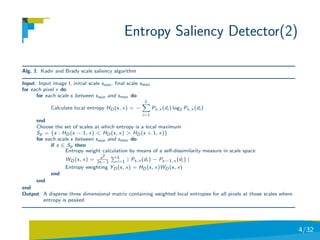
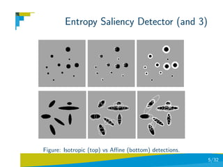
2) An entropy saliency detector is proposed that uses local entropy calculations at multiple scales to identify salient regions. Scale-space analysis allows detection of salient regions without prior knowledge of scale.
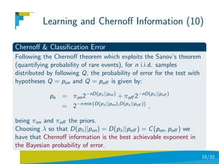
3) Techniques including Chernoff information and Kullback-Leibler divergence are discussed for learning distributions of image categories and defining thresholds to filter regions, reducing computational costs of interest point detection and description.

![Interest Points
Background.From the classical Harris detector, a big bang of
interest-point detectors ensuring some sort of invariance to
zoom/scale, rotation and perspective distortion has emerged since
the proposal of SIFT detector and descriptors [Lowe,04].
These detectors, typically including a multi-scale analysis of the
image, include Harris Affine, MSER [Matas et al,02] and SURF [Bay
et al,08].The need of an intensive comparison of different detectors
(and descriptors) mainly in terms of spatio-temporal stability
(repeatability, distinctiveness and robustness) is yet a classic
challenge [Mikolajczyk et al, 05].
Stability experiments are key to predict the future behavior of the
dectector/descriptor in subsequent tasks (bag-of-words recognition,
matching,...)
2/32](https://image.slidesharecdn.com/l2interest-pointscvpr-110515221933-phpapp02/85/CVPR2010-Advanced-ITinCVPR-in-a-Nutshell-part-2-Interest-Points-2-320.jpg)
![Entropy Saliency Detector
Local Saliency, in contrast to global one [Ullman, 96], means local
distinctiveness (outstanding/popout pixel distributions over the
image) [Julesz,81][Nothdurft,00].
In Computer Vision, a mild IT definition of local saliency is linked to
visual unpredictability [Kadir and Brady,01]. Then a salient region is
locally unpredictible (measured by entropy) and this is consistent
with a peak of entropy in scale-space.
Scale-space analysis is key because we do not know the scale of
regions beforehand. In addition, isotropic detections may be
extended to affine detectors with an extra computational cost. (see
Alg. 1).
3/32](https://image.slidesharecdn.com/l2interest-pointscvpr-110515221933-phpapp02/85/CVPR2010-Advanced-ITinCVPR-in-a-Nutshell-part-2-Interest-Points-3-320.jpg)
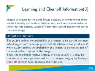
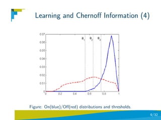
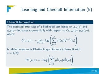
![Learning and Chernoff Information
Scale-space analysis, is, thus, one of the bottlenecks of the process.
However, having a prior knowledge of the statistics of the images
being analyzed it is possible to discard a significant number of
pixels, and thus, avoid scale-space analysis.
Working hypothesis
If the local distribution around a pixel at a scale smax is highly
homogeneous (low entropy) one may assume that for scales
s < smax it will happen the same. Thus, scale-space peaks will not
exist in this range of scales.[Suau and Escolano,08].
Inspired in statistical detection of edges [Konishi et al.,03] and
contours [Cazorla & Escolano, 03] and also in contour grouping
[Cazorla et al.,02].
6/32](https://image.slidesharecdn.com/l2interest-pointscvpr-110515221933-phpapp02/85/CVPR2010-Advanced-ITinCVPR-in-a-Nutshell-part-2-Interest-Points-6-320.jpg)
![Learning and Chernoff Information(2)
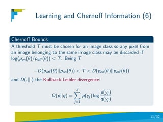
Relative entropy and threshold, a basic procedure consists of
computing the ratio between the entropy at smax and the maximum
of entropies for all pixels at their smax
Filtering by homogeneity along scale-space
1. Calculate the local entropy HD for each pixel at scale smax .
2. Select an entropy threshold σ ∈ [0, 1].
HD (x,smax )
3. X = {x | maxx {HD (x,smax )} > σ}
4. Apply scale saliency algorithm only to those pixels x ∈ X .
What is the optimal threshold σ?
7/32](https://image.slidesharecdn.com/l2interest-pointscvpr-110515221933-phpapp02/85/CVPR2010-Advanced-ITinCVPR-in-a-Nutshell-part-2-Interest-Points-7-320.jpg)
![Coarse-to-fine Visual Localization
Problem Statement
A 6DOF SLAM method has built a 3D+2D map of an
indoor/outdoor environment [Lozano et al, 09].
We have manually marked 6 environments and trained a
minimal complexity supervised classifier (see next lesson) for
performing coarse localization.
We got the statistics from the images of each environment in
order to infer their respective pon and poff distributions and
hence their Chernoff information and T bounds.
Once a test image is submitted it is classified and filtered
according to Chernoff information. Then the keypoints are
computed.
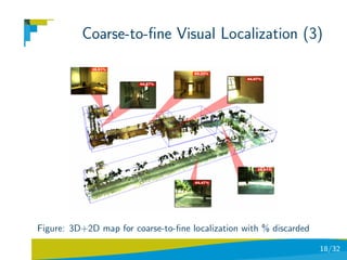
16/32](https://image.slidesharecdn.com/l2interest-pointscvpr-110515221933-phpapp02/85/CVPR2010-Advanced-ITinCVPR-in-a-Nutshell-part-2-Interest-Points-16-320.jpg)
![Coarse-to-fine Visual Localization (2)
Problem Statement (cont)
Using the SIFT descriptors of the keypoints and the GTM
algorithm [Aguilar et al, 09] we match the image with a
structural + appearance prototype previously unsupervisedly
learned through an EM-algorithm.
The prototype tells us what is the sub-environment to which
the image belongs.
In order to perform fine localization we match the image with
the structure and appearance off all images assigned to a given
sub-enviromnent and then select the one with highest
likelihood.
See more in the Feature-selection lesson.
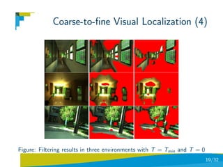
17/32](https://image.slidesharecdn.com/l2interest-pointscvpr-110515221933-phpapp02/85/CVPR2010-Advanced-ITinCVPR-in-a-Nutshell-part-2-Interest-Points-17-320.jpg)
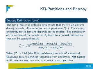
![KD-Partitions and Entropy
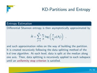
Data Partitions and Density Estimation
Let X be a d-dimensional random variable, and f (x) its pdf. Let
A = {Aj |j = 1, . . . , m} be a partition of X for which Ai ∩ Aj = ∅ if
i = j and j Aj = X . Then, we have [Stowell& Plumbley, 09]:
Aj f (x) nj
fAj = ˆ
fAj (x) = ,
µ(Aj ) nµ(Aj )
where fAj approximates f (x) in each cell, µ(Aj ) is the d-dimensional
volume of Aj . If f (x) is unknown and we are given a set of samples
X = {x1 , . . . , xn } from it, being xi ∈ Rd , we can approximate the
probability of f (x) in each cell as pj = nj /n, where nj is the number
of samples in cell Aj .
20/32](https://image.slidesharecdn.com/l2interest-pointscvpr-110515221933-phpapp02/85/CVPR2010-Advanced-ITinCVPR-in-a-Nutshell-part-2-Interest-Points-20-320.jpg)
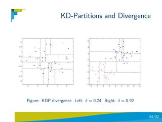
![KD-Partitions and Divergence
KDP Total-Variation Divergence
The total variation distance [Denuit and Bellegem,01] between two
probability measures P and Q for a finite alphabet, is given by:
1
δ(P, Q) = |P(x) − Q(x)| .
2 x
Then, the divergence is simply formulated as:
p
1 nx,j no,j
δ(P, Q) = |pj −qj | ∈ [0, 1], p(Aj ) = = pj p(Aj ) = = qj
2 nx no
j=1
where pi and pj are the proportion of samples of P and Q in cell Aj .
23/32](https://image.slidesharecdn.com/l2interest-pointscvpr-110515221933-phpapp02/85/CVPR2010-Advanced-ITinCVPR-in-a-Nutshell-part-2-Interest-Points-23-320.jpg)
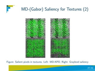
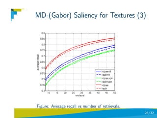
![MD-(Gabor) Saliency for Textures
KDP Total-Variation Divergence
Use Brodatz dataset (111 textures and 9 images per category:
999 images).
Use 15 Gabor filters for obtaining multi-dimensional data.
Both graylevel saliency and MD saliency are tuned to obtain
150 salient points.
Use each image in the database as query image.
Use: saliency with only RIFT, only spin images, and combining
RIFT and spin images.
retrieval-recall results strongly influenced by the type of
descriptor used [Suau & Escolano,10].
26/32](https://image.slidesharecdn.com/l2interest-pointscvpr-110515221933-phpapp02/85/CVPR2010-Advanced-ITinCVPR-in-a-Nutshell-part-2-Interest-Points-26-320.jpg)
![References
[Lowe,04] Lowe, D. (2004). Distinctive image features from scale
invariant keypoints. International Journal of Computer Vision,
60(2):91–110
[Matas et al,02] Matas, J., Chum, O., Urban, M., and Pajdla, T.
(2004). Ro- bust wide baseline stereo from maximally stable extremal
regions. Image and Vision Computing, 22(10):761–767
[Mikolajczyk et al, 05] Mikolajczyk, K., Tuytelaars, T., Schmid, C.,
Zisserman, A., Matas, J., Schaffalitzky, F., Kadir, T., and Gool, L. V.
(2005). A comparison of afne region detectors. International Journal
of Computer Vision, 65(1/2):43–72
[Ullman,96] High-level Vision, MIT Press, 1996
29/32](https://image.slidesharecdn.com/l2interest-pointscvpr-110515221933-phpapp02/85/CVPR2010-Advanced-ITinCVPR-in-a-Nutshell-part-2-Interest-Points-29-320.jpg)
![References (2)
[Julesz,81] Julesz, B. (1981). Textons, the Elements of Texture
Perception, and their Interactions. Nature 290 (5802): 91–97
[Nothdurft,00] Nothdurft, H.C. Salience from feature contrast:
variations with texture density. Vision Research 40 (2000): 3181–3200
[Kadir and Brady,01] Kadir, T. and Brady, M. (2001). Scale, saliency
and image description. International Journal of Computer Vision,
45(2):83–105
[Suau and Escolano,08] Suau, P., Escolano, F. (2008) Bayesian
Optimization of the Scale Saliency Filter. Image and Vision
Computing, 26(9), pp. 1207–1218
30/32](https://image.slidesharecdn.com/l2interest-pointscvpr-110515221933-phpapp02/85/CVPR2010-Advanced-ITinCVPR-in-a-Nutshell-part-2-Interest-Points-30-320.jpg)
![References (3)
[Konishi et al.,03] Konishi, S., Yuille, A. L., Coughlan, J. M., and
Zhu, S. C. (2003). Statistical edge detection: learning and evaluating
edge cues. IEEE Trans. on PAMI, 25(1):57–74
[Cazorla & Escolano] Cazorla, M. and Escolano, F. (2003). Two
Bayesian methods for junction detection. IEEE Transactions on
Image Processing, 12(3):317–327
[Cazorla et al.,02] Cazorla, M., Escolano, F., Gallardo, D., and Rizo,
R. (2002). Junction detection and grouping with probabilistic edge
models and Bayesian A*. Pattern Recognition, 35(9):1869–1881
[Lozano et al, 09] Lozano M,A., Escolano, F., Bonev, B., Suau, P.,
Aguilar, W., S´ez, J.M., Cazorla, M. (2009). Region and constell.
a
based categorization of images with unsupervised graph learning.
Image Vision Comput. 27(7): 960–978
31/32](https://image.slidesharecdn.com/l2interest-pointscvpr-110515221933-phpapp02/85/CVPR2010-Advanced-ITinCVPR-in-a-Nutshell-part-2-Interest-Points-31-320.jpg)
![References (4)
[Aguilar et al, 09] Aguilar, W., Frauel Y., Escolano, F., Martnez-Prez,
M.E., Espinosa-Romero, A., Lozano, M.A. (2009) A robust Graph
Transformation Matching for non-rigid registration. Image Vision
Comput. 27(7): 897–910
[Stowell& Plumbley, 09] Stowell, D. and Plumbley, M. D. (2009).
Fast multidimensional entropy estimation by k-d partitioning. IEEE
Signal Processing Letters, 16(6):537–540
[Suau & Escolano,10] Suau, P., Escolano, F. (2010). Analysis of the
Multi-Dimensional Scale Saliency Algorithm and its Application to
Texture Categorization, SSPR’2010 (accepted)
32/32](https://image.slidesharecdn.com/l2interest-pointscvpr-110515221933-phpapp02/85/CVPR2010-Advanced-ITinCVPR-in-a-Nutshell-part-2-Interest-Points-32-320.jpg)