Download to read offline


![Introduction IID Monte Carlo Low Discrepancy Bayesian Cubature Summary References
Amy (an applied mathematician) wants to compute
option price =
ż
Rd
payoff(x)
e´xT
Σ´1
x/2
(2π)d/2 |Σ|1/2
looooooomooooooon
PDF of Brownian motion at d times
dx
payoff(x) = max
1
d
dÿ
k=1
Sk(xk) ´ K, 0 e´rT
Sk(xk) = S0e(r´σ2
/2)tk+σxk
= stock price at time tk = kT/d
d, S0, K, T, r, σ arbitrary, but known
Σ = (T/d) min(k, l)
d
k,l=1
Sue (a statistician) wants to compute
Gaussian probability =
ż
[a,b]
e´xT
Σ´1
x/2
(2π)d/2 |Σ|1/2
dx
a, b, Σ arbitrary, but known
2/23](https://image.slidesharecdn.com/mines2017apriltalk-170406043746/85/Mines-April-2017-Colloquium-3-320.jpg)
![Introduction IID Monte Carlo Low Discrepancy Bayesian Cubature Summary References
Amy Suggests Rectangular Grids & Product Rules
ż 1
0
f(x) dx ´
1
m
mÿ
i=1
f
2i ´ 1
2m
= O(m´2
), so
ż
[0,1]d
f(x) dx
´
1
2m
mÿ
i1=1
¨ ¨ ¨
mÿ
id=1
f
2i1 ´ 1
2m
, . . . ,
2id ´ 1
2m
= O(m´2
) = O(n´2/d
)
assuming partial derivatives of up to order 2 in each direction exist.
3/23](https://image.slidesharecdn.com/mines2017apriltalk-170406043746/85/Mines-April-2017-Colloquium-4-320.jpg)
![Introduction IID Monte Carlo Low Discrepancy Bayesian Cubature Summary References
Amy Suggests Rectangular Grids & Product Rules
ż 1
0
f(x) dx ´
1
m
mÿ
i=1
f
2i ´ 1
2m
= O(m´2
), so
ż
[0,1]d
f(x) dx
´
1
2m
mÿ
i1=1
¨ ¨ ¨
mÿ
id=1
f
2i1 ´ 1
2m
, . . . ,
2id ´ 1
2m
= O(m´2
) = O(n´2/d
)
assuming partial derivatives of up to order 2 in each direction exist.
3/23](https://image.slidesharecdn.com/mines2017apriltalk-170406043746/85/Mines-April-2017-Colloquium-5-320.jpg)
![Introduction IID Monte Carlo Low Discrepancy Bayesian Cubature Summary References
Amy Suggests Rectangular Grids & Product Rules
ż 1
0
f(x) dx ´
1
m
mÿ
i=1
f
2i ´ 1
2m
= O(m´2
), so
ż
[0,1]d
f(x) dx
´
1
2m
mÿ
i1=1
¨ ¨ ¨
mÿ
id=1
f
2i1 ´ 1
2m
, . . . ,
2id ´ 1
2m
= O(m´2
) = O(n´2/d
)
assuming partial derivatives of up to order 2 in each direction exist.
Computational cost is prohibitive for large dimensions, d:
d 1 2 5 10 100
m = 8, n = 8d
8 64 3.3E4 1.0E9 2.0E90
Product rules are a bad idea unless d is small.
3/23](https://image.slidesharecdn.com/mines2017apriltalk-170406043746/85/Mines-April-2017-Colloquium-6-320.jpg)

![Introduction IID Monte Carlo Low Discrepancy Bayesian Cubature Summary References
Sue Suggests IID Monte Carlo
µ = E[f(X)] =
ż
Rd
f(x) ρ(x) dx
« ^µn =
1
n
nÿ
i=1
f(xi), xi
IID
„ ρ
P[|µ ´ ^µn| ď errn] « 99%
for errn =
2.58 ˆ 1.2^σ
?
n
by the Central Limit Theorem (CLT),
where ^σ2
is the sample variance. But the CLT is only an asymptotic result, and
1.2^σ may be an overly optimistic upper bound on σ.
5/23](https://image.slidesharecdn.com/mines2017apriltalk-170406043746/85/Mines-April-2017-Colloquium-8-320.jpg)
![Introduction IID Monte Carlo Low Discrepancy Bayesian Cubature Summary References
Sue Suggests IID Monte Carlo
µ = E[f(X)] =
ż
Rd
f(x) ρ(x) dx
« ^µn =
1
n
nÿ
i=1
f(xi), xi
IID
„ ρ
P[|µ ´ ^µn| ď errn] « 99%
for errn =
2.58 ˆ 1.2^σ
?
n
by the Central Limit Theorem (CLT),
where ^σ2
is the sample variance. But the CLT is only an asymptotic result, and
1.2^σ may be an overly optimistic upper bound on σ.
A Berry-Esseen Inequality, Cantelli’s Inequality, and an assumed upper bound on
the kurtosis can be used to provide a rigorous error bound (H. et al., 2013; Jiang,
2016). More
5/23](https://image.slidesharecdn.com/mines2017apriltalk-170406043746/85/Mines-April-2017-Colloquium-9-320.jpg)
![Introduction IID Monte Carlo Low Discrepancy Bayesian Cubature Summary References
Sue’s Gaussian Probability
µ =
ż
[a,b]
exp ´1
2 tT
Σ´1
t
a
(2π)d det(Σ)
dt
affine
=
ż
[0,1]d
f(x) dx
For some typical choice of a, b, Σ, d = 3; µ « 0.6763
Rel. Error Median Worst 10% Worst 10%
Tolerance Method Error Accuracy n Time (s)
1E´2 IID Affine 7E´4 100% 1.5E6 1.8E´1
6/23](https://image.slidesharecdn.com/mines2017apriltalk-170406043746/85/Mines-April-2017-Colloquium-10-320.jpg)
![Introduction IID Monte Carlo Low Discrepancy Bayesian Cubature Summary References
Amy Suggests a Variable Transformation
µ =
ż
[a,b]
exp ´1
2 tT
Σ´1
t
a
(2π)d det(Σ)
dt
Genz (1993)
=
ż
[0,1]d´1
f(x) dx
For some typical choice of a, b, Σ, d = 3; µ « 0.6763
Rel. Error Median Worst 10% Worst 10%
Tolerance Method Error Accuracy n Time (s)
1E´2 IID Affine 7E´4 100% 1.5E6 1.8E´1
1E´2 IID Genz 4E´4 100% 8.1E4 1.9E´2
6/23](https://image.slidesharecdn.com/mines2017apriltalk-170406043746/85/Mines-April-2017-Colloquium-11-320.jpg)
![Introduction IID Monte Carlo Low Discrepancy Bayesian Cubature Summary References
IID Monte Carlo Is Slow
µ =
ż
[a,b]
exp ´1
2 tT
Σ´1
t
a
(2π)d det(Σ)
dt
Genz (1993)
=
ż
[0,1]d´1
f(x) dx
For some typical choice of a, b, Σ, d = 3; µ « 0.6763
Rel. Error Median Worst 10% Worst 10%
Tolerance Method Error Accuracy n Time (s)
1E´2 IID Affine 7E´4 100% 1.5E6 1.8E´1
1E´2 IID Genz 4E´4 100% 8.1E4 1.9E´2
1E´3 IID Genz 7E´5 100% 2.0E6 3.8E´1
6/23](https://image.slidesharecdn.com/mines2017apriltalk-170406043746/85/Mines-April-2017-Colloquium-12-320.jpg)
![Introduction IID Monte Carlo Low Discrepancy Bayesian Cubature Summary References
Sue Suggests IID Monte Carlo
µ = E[f(X)] =
ż
Rd
f(x) ρ(x) dx
« ^µn =
1
n
nÿ
i=1
f(xi), xi
IID
„ ρ
P[|µ ´ ^µn| ď errn] « 99%
for errn =
2.58 ˆ 1.2^σ
?
n
by the Central Limit Theorem (CLT),
where ^σ2
is the sample variance. But the CLT is only an asymptotic result, and
1.2^σ may be an overly optimistic upper bound on σ.
A Berry-Esseen Inequality, Cantelli’s Inequality, and an assumed upper bound on
the kurtosis can be used to provide a rigorous error bound (H. et al., 2013; Jiang,
2016). More
7/23](https://image.slidesharecdn.com/mines2017apriltalk-170406043746/85/Mines-April-2017-Colloquium-13-320.jpg)
![Introduction IID Monte Carlo Low Discrepancy Bayesian Cubature Summary References
Amy Suggests More Even Sampling than IID
µ =
ż
[0,1]d
f(x) dx « ^µn =
1
n
nÿ
i=1
f(xi),
xi Sobol’ (Dick and Pillichshammer, 2010)
Normally n should be a power of 2
8/23](https://image.slidesharecdn.com/mines2017apriltalk-170406043746/85/Mines-April-2017-Colloquium-14-320.jpg)
![Introduction IID Monte Carlo Low Discrepancy Bayesian Cubature Summary References
Amy Suggests More Even Sampling than IID
µ =
ż
[0,1]d
f(x) dx « ^µn =
1
n
nÿ
i=1
f(xi),
xi Sobol’ (Dick and Pillichshammer, 2010)
Normally n should be a power of 2
8/23](https://image.slidesharecdn.com/mines2017apriltalk-170406043746/85/Mines-April-2017-Colloquium-15-320.jpg)
![Introduction IID Monte Carlo Low Discrepancy Bayesian Cubature Summary References
Amy Suggests More Even Sampling than IID
µ =
ż
[0,1]d
f(x) dx « ^µn =
1
n
nÿ
i=1
f(xi),
xi Sobol’ (Dick and Pillichshammer, 2010)
Normally n should be a power of 2
8/23](https://image.slidesharecdn.com/mines2017apriltalk-170406043746/85/Mines-April-2017-Colloquium-16-320.jpg)
![Introduction IID Monte Carlo Low Discrepancy Bayesian Cubature Summary References
Amy Suggests More Even Sampling than IID
µ =
ż
[0,1]d
f(x) dx « ^µn =
1
n
nÿ
i=1
f(xi),
xi Sobol’ (Dick and Pillichshammer, 2010)
Normally n should be a power of 2
8/23](https://image.slidesharecdn.com/mines2017apriltalk-170406043746/85/Mines-April-2017-Colloquium-17-320.jpg)
![Introduction IID Monte Carlo Low Discrepancy Bayesian Cubature Summary References
Amy Suggests More Even Sampling than IID
µ =
ż
[0,1]d
f(x) dx « ^µn =
1
n
nÿ
i=1
f(xi),
xi Sobol’ (Dick and Pillichshammer, 2010)
Normally n should be a power of 2
8/23](https://image.slidesharecdn.com/mines2017apriltalk-170406043746/85/Mines-April-2017-Colloquium-18-320.jpg)
![Introduction IID Monte Carlo Low Discrepancy Bayesian Cubature Summary References
Amy Suggests More Even Sampling than IID
µ =
ż
[0,1]d
f(x) dx « ^µn =
1
n
nÿ
i=1
f(xi),
xi Sobol’ (Dick and Pillichshammer, 2010)
Normally n should be a power of 2
8/23](https://image.slidesharecdn.com/mines2017apriltalk-170406043746/85/Mines-April-2017-Colloquium-19-320.jpg)
![Introduction IID Monte Carlo Low Discrepancy Bayesian Cubature Summary References
Amy Suggests More Even Sampling than IID
µ =
ż
[0,1]d
f(x) dx « ^µn =
1
n
nÿ
i=1
f(xi),
xi Sobol’ (Dick and Pillichshammer, 2010)
Normally n should be a power of 2
8/23](https://image.slidesharecdn.com/mines2017apriltalk-170406043746/85/Mines-April-2017-Colloquium-20-320.jpg)
![Introduction IID Monte Carlo Low Discrepancy Bayesian Cubature Summary References
Amy Suggests More Even Sampling than IID
µ =
ż
[0,1]d
f(x) dx « ^µn =
1
n
nÿ
i=1
f(xi),
xi Sobol’ (Dick and Pillichshammer, 2010)
Normally n should be a power of 2
8/23](https://image.slidesharecdn.com/mines2017apriltalk-170406043746/85/Mines-April-2017-Colloquium-21-320.jpg)
![Introduction IID Monte Carlo Low Discrepancy Bayesian Cubature Summary References
Amy Suggests More Even Sampling than IID
µ =
ż
[0,1]d
f(x) dx « ^µn =
1
n
nÿ
i=1
f(xi),
xi Sobol’ (Dick and Pillichshammer, 2010)
Normally n should be a power of 2
8/23](https://image.slidesharecdn.com/mines2017apriltalk-170406043746/85/Mines-April-2017-Colloquium-22-320.jpg)
![Introduction IID Monte Carlo Low Discrepancy Bayesian Cubature Summary References
Amy Suggests More Even Sampling than IID
µ =
ż
[0,1]d
f(x) dx « ^µn =
1
n
nÿ
i=1
f(xi),
xi Sobol’ (Dick and Pillichshammer, 2010)
Normally n should be a power of 2
8/23](https://image.slidesharecdn.com/mines2017apriltalk-170406043746/85/Mines-April-2017-Colloquium-23-320.jpg)
![Introduction IID Monte Carlo Low Discrepancy Bayesian Cubature Summary References
Amy Suggests More Even Sampling than IID
µ =
ż
[0,1]d
f(x) dx « ^µn =
1
n
nÿ
i=1
f(xi),
xi Sobol’ (Dick and Pillichshammer, 2010)
Normally n should be a power of 2
8/23](https://image.slidesharecdn.com/mines2017apriltalk-170406043746/85/Mines-April-2017-Colloquium-24-320.jpg)
![Introduction IID Monte Carlo Low Discrepancy Bayesian Cubature Summary References
Amy Suggests More Even Sampling than IID
µ =
ż
[0,1]d
f(x) dx « ^µn =
1
n
nÿ
i=1
f(xi),
xi Sobol’ (Dick and Pillichshammer, 2010)
Normally n should be a power of 2
8/23](https://image.slidesharecdn.com/mines2017apriltalk-170406043746/85/Mines-April-2017-Colloquium-25-320.jpg)
![Introduction IID Monte Carlo Low Discrepancy Bayesian Cubature Summary References
Amy Suggests More Even Sampling than IID
µ =
ż
[0,1]d
f(x) dx « ^µn =
1
n
nÿ
i=1
f(xi),
xi Sobol’ (Dick and Pillichshammer, 2010)
Normally n should be a power of 2
8/23](https://image.slidesharecdn.com/mines2017apriltalk-170406043746/85/Mines-April-2017-Colloquium-26-320.jpg)
![Introduction IID Monte Carlo Low Discrepancy Bayesian Cubature Summary References
Amy Suggests More Even Sampling than IID
µ =
ż
[0,1]d
f(x) dx « ^µn =
1
n
nÿ
i=1
f(xi),
xi Sobol’ (Dick and Pillichshammer, 2010)
Normally n should be a power of 2
8/23](https://image.slidesharecdn.com/mines2017apriltalk-170406043746/85/Mines-April-2017-Colloquium-27-320.jpg)
![Introduction IID Monte Carlo Low Discrepancy Bayesian Cubature Summary References
Amy Suggests More Even Sampling than IID
µ =
ż
[0,1]d
f(x) dx « ^µn =
1
n
nÿ
i=1
f(xi),
xi Sobol’ (Dick and Pillichshammer, 2010)
Assume f P Hilbert space H with
reproducing kernel K (H., 1998)
µ(f) ´ ^µ(f) = xerr-rep, fy
= cos(err-rep, f) ˆ err-rep Hlooooomooooon
discrepancy
=O(n´1+
)
ˆ f H
err-rep
2
H =
ż
[0,1]2d
K(x, t) dxdt ´
2
n
nÿ
i=1
ż
[0,1]d
K(xi, t) dt +
1
n2
nÿ
i,j=1
K(xi, xj)
Adaptive stopping criteria developed (H. and Jiménez Rugama, 2016; Jiménez
Rugama and H., 2016; H. et al., 2017+). More
8/23](https://image.slidesharecdn.com/mines2017apriltalk-170406043746/85/Mines-April-2017-Colloquium-28-320.jpg)
![Introduction IID Monte Carlo Low Discrepancy Bayesian Cubature Summary References
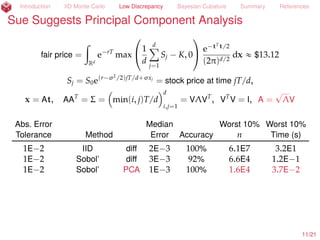
Sobol’ Sampling Converges Faster
µ =
ż
[a,b]
exp ´1
2 tT
Σ´1
t
a
(2π)d det(Σ)
dt
Genz (1993)
=
ż
[0,1]d´1
f(x) dx
For some typical choice of a, b, Σ, d = 3; µ « 0.6763
Rel. Error Median Worst 10% Worst 10%
Tolerance Method Error Accuracy n Time (s)
1E´2 IID Affine 7E´4 100% 1.5E6 1.8E´1
1E´2 IID Genz 4E´4 100% 8.1E4 1.9E´2
1E´2 Sobol’ Genz 3E´4 100% 1.0E3 4.6E´3
1E´3 IID Genz 7E´5 100% 2.0E6 3.8E´1
1E´3 Sobol’ Genz 2E´4 100% 2.0E3 6.1E´3
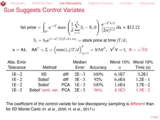
9/23](https://image.slidesharecdn.com/mines2017apriltalk-170406043746/85/Mines-April-2017-Colloquium-29-320.jpg)
![Introduction IID Monte Carlo Low Discrepancy Bayesian Cubature Summary References
Sue Randomizes Even Sampling
µ =
ż
[0,1]d
f(x) dx « ^µn =
1
n
nÿ
i=1
f(xi),
xi scrambled Sobol’ (Owen, 1997a; 1997b)
Normally n should be a power of 2
E(^µ) = µ no bias
std(^µ) = n´1.5+
for scrambled Sobol’
10/23](https://image.slidesharecdn.com/mines2017apriltalk-170406043746/85/Mines-April-2017-Colloquium-30-320.jpg)
![Introduction IID Monte Carlo Low Discrepancy Bayesian Cubature Summary References
Sue Randomizes Even Sampling
µ =
ż
[0,1]d
f(x) dx « ^µn =
1
n
nÿ
i=1
f(xi),
xi scrambled Sobol’ (Owen, 1997a; 1997b)
Normally n should be a power of 2
E(^µ) = µ no bias
std(^µ) = n´1.5+
for scrambled Sobol’
10/23](https://image.slidesharecdn.com/mines2017apriltalk-170406043746/85/Mines-April-2017-Colloquium-31-320.jpg)
![Introduction IID Monte Carlo Low Discrepancy Bayesian Cubature Summary References
Sue Randomizes Even Sampling
µ =
ż
[0,1]d
f(x) dx « ^µn =
1
n
nÿ
i=1
f(xi),
xi scrambled Sobol’ (Owen, 1997a; 1997b)
Normally n should be a power of 2
E(^µ) = µ no bias
std(^µ) = n´1.5+
for scrambled Sobol’
10/23](https://image.slidesharecdn.com/mines2017apriltalk-170406043746/85/Mines-April-2017-Colloquium-32-320.jpg)
![Introduction IID Monte Carlo Low Discrepancy Bayesian Cubature Summary References
Sue Randomizes Even Sampling
µ =
ż
[0,1]d
f(x) dx « ^µn =
1
n
nÿ
i=1
f(xi),
xi scrambled Sobol’ (Owen, 1997a; 1997b)
Normally n should be a power of 2
E(^µ) = µ no bias
std(^µ) = n´1.5+
for scrambled Sobol’
10/23](https://image.slidesharecdn.com/mines2017apriltalk-170406043746/85/Mines-April-2017-Colloquium-33-320.jpg)
![Introduction IID Monte Carlo Low Discrepancy Bayesian Cubature Summary References
Sue Randomizes Even Sampling
µ =
ż
[0,1]d
f(x) dx « ^µn =
1
n
nÿ
i=1
f(xi),
xi scrambled Sobol’ (Owen, 1997a; 1997b)
Normally n should be a power of 2
E(^µ) = µ no bias
std(^µ) = n´1.5+
for scrambled Sobol’
10/23](https://image.slidesharecdn.com/mines2017apriltalk-170406043746/85/Mines-April-2017-Colloquium-34-320.jpg)
![Introduction IID Monte Carlo Low Discrepancy Bayesian Cubature Summary References
Sue Randomizes Even Sampling
µ =
ż
[0,1]d
f(x) dx « ^µn =
1
n
nÿ
i=1
f(xi),
xi scrambled Sobol’ (Owen, 1997a; 1997b)
Normally n should be a power of 2
E(^µ) = µ no bias
std(^µ) = n´1.5+
for scrambled Sobol’
10/23](https://image.slidesharecdn.com/mines2017apriltalk-170406043746/85/Mines-April-2017-Colloquium-35-320.jpg)
![Introduction IID Monte Carlo Low Discrepancy Bayesian Cubature Summary References
Sue Randomizes Even Sampling
µ =
ż
[0,1]d
f(x) dx « ^µn =
1
n
nÿ
i=1
f(xi),
xi scrambled Sobol’ (Owen, 1997a; 1997b)
Normally n should be a power of 2
E(^µ) = µ no bias
std(^µ) = n´1.5+
for scrambled Sobol’
10/23](https://image.slidesharecdn.com/mines2017apriltalk-170406043746/85/Mines-April-2017-Colloquium-36-320.jpg)
![Introduction IID Monte Carlo Low Discrepancy Bayesian Cubature Summary References
Sue Randomizes Even Sampling
µ =
ż
[0,1]d
f(x) dx « ^µn =
1
n
nÿ
i=1
f(xi),
xi scrambled Sobol’ (Owen, 1997a; 1997b)
Normally n should be a power of 2
E(^µ) = µ no bias
std(^µ) = n´1.5+
for scrambled Sobol’
10/23](https://image.slidesharecdn.com/mines2017apriltalk-170406043746/85/Mines-April-2017-Colloquium-37-320.jpg)
![Introduction IID Monte Carlo Low Discrepancy Bayesian Cubature Summary References
Sue Randomizes Even Sampling
µ =
ż
[0,1]d
f(x) dx « ^µn =
1
n
nÿ
i=1
f(xi),
xi scrambled Sobol’ (Owen, 1997a; 1997b)
Normally n should be a power of 2
E(^µ) = µ no bias
std(^µ) = n´1.5+
for scrambled Sobol’
10/23](https://image.slidesharecdn.com/mines2017apriltalk-170406043746/85/Mines-April-2017-Colloquium-38-320.jpg)
![Introduction IID Monte Carlo Low Discrepancy Bayesian Cubature Summary References
Sue Randomizes Even Sampling
µ =
ż
[0,1]d
f(x) dx « ^µn =
1
n
nÿ
i=1
f(xi),
xi scrambled Sobol’ (Owen, 1997a; 1997b)
Normally n should be a power of 2
E(^µ) = µ no bias
std(^µ) = n´1.5+
for scrambled Sobol’
10/23](https://image.slidesharecdn.com/mines2017apriltalk-170406043746/85/Mines-April-2017-Colloquium-39-320.jpg)
![Introduction IID Monte Carlo Low Discrepancy Bayesian Cubature Summary References
Sue Randomizes Even Sampling
µ =
ż
[0,1]d
f(x) dx « ^µn =
1
n
nÿ
i=1
f(xi),
xi scrambled Sobol’ (Owen, 1997a; 1997b)
Normally n should be a power of 2
E(^µ) = µ no bias
std(^µ) = n´1.5+
for scrambled Sobol’
10/23](https://image.slidesharecdn.com/mines2017apriltalk-170406043746/85/Mines-April-2017-Colloquium-40-320.jpg)
![Introduction IID Monte Carlo Low Discrepancy Bayesian Cubature Summary References
Sue Randomizes Even Sampling
µ =
ż
[0,1]d
f(x) dx « ^µn =
1
n
nÿ
i=1
f(xi),
xi scrambled Sobol’ (Owen, 1997a; 1997b)
Normally n should be a power of 2
E(^µ) = µ no bias
std(^µ) = n´1.5+
for scrambled Sobol’
10/23](https://image.slidesharecdn.com/mines2017apriltalk-170406043746/85/Mines-April-2017-Colloquium-41-320.jpg)
![Introduction IID Monte Carlo Low Discrepancy Bayesian Cubature Summary References
Sue Randomizes Even Sampling
µ =
ż
[0,1]d
f(x) dx « ^µn =
1
n
nÿ
i=1
f(xi),
xi scrambled Sobol’ (Owen, 1997a; 1997b)
Normally n should be a power of 2
E(^µ) = µ no bias
std(^µ) = n´1.5+
for scrambled Sobol’
10/23](https://image.slidesharecdn.com/mines2017apriltalk-170406043746/85/Mines-April-2017-Colloquium-42-320.jpg)
![Introduction IID Monte Carlo Low Discrepancy Bayesian Cubature Summary References
Sue Randomizes Even Sampling
µ =
ż
[0,1]d
f(x) dx « ^µn =
1
n
nÿ
i=1
f(xi),
xi scrambled Sobol’ (Owen, 1997a; 1997b)
Normally n should be a power of 2
E(^µ) = µ no bias
std(^µ) = n´1.5+
for scrambled Sobol’
10/23](https://image.slidesharecdn.com/mines2017apriltalk-170406043746/85/Mines-April-2017-Colloquium-43-320.jpg)
![Introduction IID Monte Carlo Low Discrepancy Bayesian Cubature Summary References
Sue Randomizes Even Sampling
µ =
ż
[0,1]d
f(x) dx « ^µn =
1
n
nÿ
i=1
f(xi),
xi scrambled Sobol’ (Owen, 1997a; 1997b)
or shifted lattice (Cranley and Patterson, 1976)
Normally n should be a power of 2
E(^µ) = µ no bias
std(^µ) = n´1+
for shifted lattices
10/23](https://image.slidesharecdn.com/mines2017apriltalk-170406043746/85/Mines-April-2017-Colloquium-44-320.jpg)
![Introduction IID Monte Carlo Low Discrepancy Bayesian Cubature Summary References
Sue Randomizes Even Sampling
µ =
ż
[0,1]d
f(x) dx « ^µn =
1
n
nÿ
i=1
f(xi),
xi scrambled Sobol’ (Owen, 1997a; 1997b)
or shifted lattice (Cranley and Patterson, 1976)
Normally n should be a power of 2
E(^µ) = µ no bias
std(^µ) = n´1+
for shifted lattices
10/23](https://image.slidesharecdn.com/mines2017apriltalk-170406043746/85/Mines-April-2017-Colloquium-45-320.jpg)
![Introduction IID Monte Carlo Low Discrepancy Bayesian Cubature Summary References
Scrambled Sobol’ Is Better
µ =
ż
[a,b]
exp ´1
2 tT
Σ´1
t
a
(2π)d det(Σ)
dt
Genz (1993)
=
ż
[0,1]d´1
f(x) dx
For some typical choice of a, b, Σ, d = 3; µ « 0.6763
Rel. Error Median Worst 10% Worst 10%
Tolerance Method Error Accuracy n Time (s)
1E´2 IID Affine 7E´4 100% 1.5E6 1.8E´1
1E´2 IID Genz 4E´4 100% 8.1E4 1.9E´2
1E´2 Sobol’ Genz 3E´4 100% 1.0E3 4.6E´3
1E´2 Scr. Sobol’ Genz 6E´5 100% 1.0E3 5.0E´3
1E´3 IID Genz 7E´5 100% 2.0E6 3.8E´1
1E´3 Sobol’ Genz 2E´4 100% 2.0E3 6.1E´3
1E´3 Scr. Sobol’ Genz 2E´5 100% 2.0E3 6.7E´3
1E´4 Scr. Sobol’ Genz 5E´7 100% 1.6E4 1.9E´2
11/23](https://image.slidesharecdn.com/mines2017apriltalk-170406043746/85/Mines-April-2017-Colloquium-46-320.jpg)


![Introduction IID Monte Carlo Low Discrepancy Bayesian Cubature Summary References
Amy Suggests Nice C
µ =
ż
Rd
f(x) ρ(x) dx « ^µn =
nÿ
i=1
wi f(xi)
Assume f „ GP(0, s2
Cθ) (Diaconis, 1988;
O’Hagan, 1991; Ritter, 2000; Rasmussen and
Ghahramani, 2003)
c0 =
ż
RdˆRd
Cθ(x, t) ρ(x)ρ(t) dxdt
c =
ż
Rd
Cθ(xi, t) ρ(x) dx
n
i=1
, C = Cθ(xi, xj)
n
i,j=1
Choosing w = wi
n
i=1
= C´1
c is optimal
P[|µ ´ ^µn| ď errn] = 99% for errn = 2.58
c
c0 ´ cTC´1c
yTC´1y
n
where y = f(xi)
n
i=1
. But, θ needs to be inferred (by MLE) More . If C is nice,
then operations involving C only require O(n log(n)) operations.
13/23](https://image.slidesharecdn.com/mines2017apriltalk-170406043746/85/Mines-April-2017-Colloquium-51-320.jpg)
![Introduction IID Monte Carlo Low Discrepancy Bayesian Cubature Summary References
Bayesian Cubature Is Promising
µ =
ż
[a,b]
exp ´1
2 tT
Σ´1
t
a
(2π)d det(Σ)
dt
Genz (1993)
=
ż
[0,1]d´1
f(x) dx
For some typical choice of a, b, Σ, d = 3; µ « 0.6763
Rel. Error Median Worst 10% Worst 10%
Tolerance Method Error Accuracy n Time (s)
1E´2 IID Affine 7E´4 100% 1.5E6 1.8E´1
1E´2 IID Genz 4E´4 100% 8.1E4 1.9E´2
1E´2 Sobol’ Genz 3E´4 100% 1.0E3 4.6E´3
1E´2 Scr. Sobol’ Genz 6E´5 100% 1.0E3 5.0E´3
1E´2 Bayes. Latt. Genz 1E´5 100% 1.0E3 3.7E´3
1E´3 IID Genz 7E´5 100% 2.0E6 3.8E´1
1E´3 Sobol’ Genz 2E´4 100% 2.0E3 6.1E´3
1E´3 Scr. Sobol’ Genz 2E´5 100% 2.0E3 6.7E´3
1E´3 Bayes. Latt. Genz 9E´6 100% 1.0E3 2.6E´3
1E´4 Scr. Sobol’ Genz 5E´7 100% 1.6E4 1.9E´2
1E´4 Bayes. Latt. Genz 5E´7 100% 8.2E3 1.3E´2
14/23](https://image.slidesharecdn.com/mines2017apriltalk-170406043746/85/Mines-April-2017-Colloquium-52-320.jpg)


![Introduction IID Monte Carlo Low Discrepancy Bayesian Cubature Summary References
References II
H., F. J. and Ll. A. Jiménez Rugama. 2016. Reliable adaptive cubature using digital sequences,
Monte Carlo and quasi-Monte Carlo methods: MCQMC, Leuven, Belgium, April 2014, pp. 367–383.
arXiv:1410.8615 [math.NA].
H., F. J., Ll. A. Jiménez Rugama, and D. Li. 2017+. Adaptive quasi-Monte Carlo methods. submitted
for publication, arXiv:1702.01491 [math.NA].
H., F. J., C. Lemieux, and A. B. Owen. 2005. Control variates for quasi-Monte Carlo, Statist. Sci. 20,
1–31.
Jiang, L. 2016. Guaranteed adaptive Monte Carlo methods for estimating means of random
variables, Ph.D. Thesis.
Jiménez Rugama, Ll. A. and F. J. H. 2016. Adaptive multidimensional integration based on rank-1
lattices, Monte Carlo and quasi-Monte Carlo methods: MCQMC, Leuven, Belgium, April 2014,
pp. 407–422. arXiv:1411.1966.
Meng, X. 2017+. Statistical paradises and paradoxes in big data. in preparation.
O’Hagan, A. 1991. Bayes-Hermite quadrature, J. Statist. Plann. Inference 29, 245–260.
Owen, A. B. 1997a. Monte Carlo variance of scrambled net quadrature, SIAM J. Numer. Anal. 34,
1884–1910.
. 1997b. Scrambled net variance for integrals of smooth functions, Ann. Stat. 25, 1541–1562.
Rasmussen, C. E. and Z. Ghahramani. 2003. Bayesian Monte Carlo, Advances in Neural Information
Processing Systems, pp. 489–496.
19/23](https://image.slidesharecdn.com/mines2017apriltalk-170406043746/85/Mines-April-2017-Colloquium-57-320.jpg)
![Introduction IID Monte Carlo Low Discrepancy Bayesian Cubature Summary References
Sue Suggests IID Monte Carlo
µ = E[f(X)] =
ż
Rd
f(x) ρ(x) dx
« ^µn =
1
n
nÿ
i=1
f(xi), xi
IID
„ ρ
P[|µ ´ ^µn| ď errn] ě 99%
for Φ ´
?
n errn /(1.2^σnσ
)
+ ∆n(´
?
n errn /(1.2^σnσ
), κmax) = 0.0025
by the Berry-Esseen Inequality,
where ^σ2
nσ
is the sample variance using an independent sample from that used to
simulate the mean, and provided that kurt(f(X)) ď κmax(nσ) (H. et al., 2013;
Jiang, 2016). Return
21/23](https://image.slidesharecdn.com/mines2017apriltalk-170406043746/85/Mines-April-2017-Colloquium-59-320.jpg)
![Introduction IID Monte Carlo Low Discrepancy Bayesian Cubature Summary References
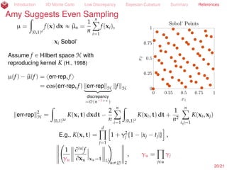
Amy Suggests More Even Sampling than IID
µ =
ż
[0,1]d
f(x) dx « ^µn =
1
n
nÿ
i=1
f(xi),
xi Sobol’ (Dick and Pillichshammer, 2010)
Assume f P Hilbert space H with
reproducing kernel K (H., 1998)
µ(f) ´ ^µ(f) = xerr-rep, fy
= cos(err-rep, f) ˆ err-rep Hlooooomooooon
discrepancy
=O(n´1+
)
ˆ f H
err-rep
2
H =
ż
[0,1]2d
K(x, t) dxdt ´
2
n
nÿ
i=1
ż
[0,1]d
K(xi, t) dt +
1
n2
nÿ
i,j=1
K(xi, xj)
E.g., K(x, t) =
dź
k=1
1 + γ2
kt1 ´ |xk ´ tk|u ,
1
γu
B|u|
f
Bxu xsu=1 L2
u‰H 2
, γu =
ź
kPu
γk
22/23](https://image.slidesharecdn.com/mines2017apriltalk-170406043746/85/Mines-April-2017-Colloquium-60-320.jpg)
![Introduction IID Monte Carlo Low Discrepancy Bayesian Cubature Summary References
Amy Suggests More Even Sampling than IID
µ =
ż
[0,1]d
f(x) dx « ^µn =
1
n
nÿ
i=1
f(xi),
xi Sobol’ (Dick and Pillichshammer, 2010)
Let pf(k)
(
k
denote the coefficients of the
Fourier Walsh expansion of f. Let tω(k)uk
be some weights. Then
µ ´ ^µn =
´
ÿ
0‰kPdual
pf(k)
! pf(k)
ω(k)
)
k 2
tω(k)u0‰kPdual 2
loooooooooooooooooooomoooooooooooooooooooon
ALNP[´1,1]
ˆ tω(k)u0‰kPdual 2loooooooooomoooooooooon
DSC(txiun
i=1)=O(n´1+ )
ˆ
#
pf(k)
ω(k)
+
k 2looooooomooooooon
VAR(f)
22/23](https://image.slidesharecdn.com/mines2017apriltalk-170406043746/85/Mines-April-2017-Colloquium-61-320.jpg)
![Introduction IID Monte Carlo Low Discrepancy Bayesian Cubature Summary References
Amy Suggests More Even Sampling than IID
µ =
ż
[0,1]d
f(x) dx « ^µn =
1
n
nÿ
i=1
f(xi),
xi Sobol’ (Dick and Pillichshammer, 2010)
Let pf(k)
(
k
denote the coefficients of the
Fourier Walsh expansion of f. Let tω(k)uk
be some weights. Then
Assuming that the pf(k) do not decay erratically as k Ñ ∞, the discrete
transform, rfn(k)
(
k
, may be used to bound the error reliably (H. and Jiménez
Rugama, 2016; Jiménez Rugama and H., 2016; H. et al., 2017+):
|µ ´ ^µn| ď errn := C(n)
ÿ
certaink
rfn(k)
Return
22/23](https://image.slidesharecdn.com/mines2017apriltalk-170406043746/85/Mines-April-2017-Colloquium-62-320.jpg)
![Introduction IID Monte Carlo Low Discrepancy Bayesian Cubature Summary References
Maximum Likelihood Estimation of the Covariance Kernel
f „ GP(0, s2
Cθ), Cθ = Cθ(xi, xj)
n
i,j=1
y = f(xi)
n
i=1
, ^µn = cT
^θ
C´1
^θ
y
^θ = argmin
θ
yT
C´1
θ y
[det(C´1
θ )]1/n
P[|µ ´ ^µn| ď errn] = 99% for errn =
2.58
?
n
b
c0,^θ ´ cT
^θ
C´1
^θ
c^θ yTC´1
^θ
y
23/23](https://image.slidesharecdn.com/mines2017apriltalk-170406043746/85/Mines-April-2017-Colloquium-63-320.jpg)
![Introduction IID Monte Carlo Low Discrepancy Bayesian Cubature Summary References
Maximum Likelihood Estimation of the Covariance Kernel
f „ GP(0, s2
Cθ), Cθ = Cθ(xi, xj)
n
i,j=1
y = f(xi)
n
i=1
, ^µn = cT
^θ
C´1
^θ
y
^θ = argmin
θ
yT
C´1
θ y
[det(C´1
θ )]1/n
P[|µ ´ ^µn| ď errn] = 99% for errn =
2.58
?
n
b
c0,^θ ´ cT
^θ
C´1
^θ
c^θ yTC´1
^θ
y
There is a de-randomized interpretation of Bayesian cubature (H., 2017+)
f P Hilbert space w/ reproducing kernel Cθ and with best interpolant rfy
Return 23/23](https://image.slidesharecdn.com/mines2017apriltalk-170406043746/85/Mines-April-2017-Colloquium-64-320.jpg)
![Introduction IID Monte Carlo Low Discrepancy Bayesian Cubature Summary References
Maximum Likelihood Estimation of the Covariance Kernel
f „ GP(0, s2
Cθ), Cθ = Cθ(xi, xj)
n
i,j=1
y = f(xi)
n
i=1
, ^µn = cT
^θ
C´1
^θ
y
^θ = argmin
θ
yT
C´1
θ y
[det(C´1
θ )]1/n
P[|µ ´ ^µn| ď errn] = 99% for errn =
2.58
?
n
b
c0,^θ ´ cT
^θ
C´1
^θ
c^θ yTC´1
^θ
y
There is a de-randomized interpretation of Bayesian cubature (H., 2017+)
f P Hilbert space w/ reproducing kernel Cθ and with best interpolant rfy
|µ ´ ^µn| ď
2.58
?
n
b
c0,^θ ´ cT
^θ
C´1
^θ
c^θ
loooooooooomoooooooooon
error representer ^θ
b
yTC´1
^θ
y
looooomooooon
rfy ^θ
if f ´ rfy ^θ
ď
2.58 rf ^θ?
n
Return 23/23](https://image.slidesharecdn.com/mines2017apriltalk-170406043746/85/Mines-April-2017-Colloquium-65-320.jpg)
![Introduction IID Monte Carlo Low Discrepancy Bayesian Cubature Summary References
Maximum Likelihood Estimation of the Covariance Kernel
f „ GP(0, s2
Cθ), Cθ = Cθ(xi, xj)
n
i,j=1
y = f(xi)
n
i=1
, ^µn = cT
^θ
C´1
^θ
y
^θ = argmin
θ
yT
C´1
θ y
[det(C´1
θ )]1/n
P[|µ ´ ^µn| ď errn] = 99% for errn =
2.58
?
n
b
c0,^θ ´ cT
^θ
C´1
^θ
c^θ yTC´1
^θ
y
There is a de-randomized interpretation of Bayesian cubature (H., 2017+)
f P Hilbert space w/ reproducing kernel Cθ and with best interpolant rfy
^θ = argmin
θ
yT
C´1
θ y
[det(C´1
θ )]1/n
= argmin
θ
vol z P Rn
: rfz θ ď rfy θ
(
|µ ´ ^µn| ď
2.58
?
n
b
c0,^θ ´ cT
^θ
C´1
^θ
c^θ
loooooooooomoooooooooon
error representer ^θ
b
yTC´1
^θ
y
looooomooooon
rfy ^θ
if f ´ rfy ^θ
ď
2.58 rf ^θ?
n
Return 23/23](https://image.slidesharecdn.com/mines2017apriltalk-170406043746/85/Mines-April-2017-Colloquium-66-320.jpg)

The document discusses various computational methods for estimating option prices and Gaussian probabilities using techniques such as Monte Carlo and cubature. It evaluates the efficiency of these methods based on dimensionality and sampling strategies, noting that traditional methods can be computationally prohibitive in higher dimensions. The authors, Amy and Sue, suggest alternatives for sampling to improve accuracy and convergence rates in computations.