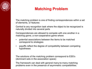
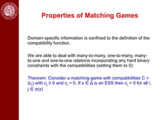
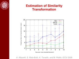
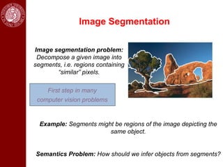
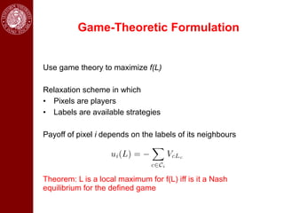
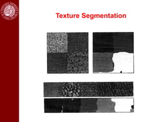
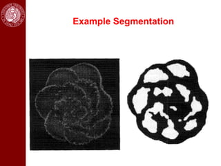
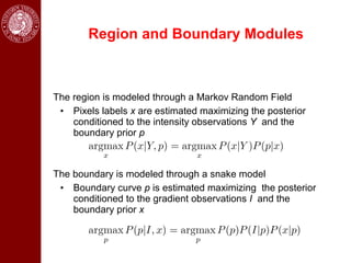
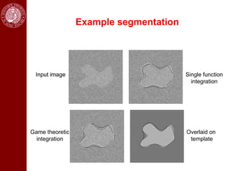
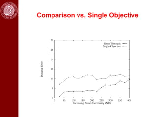
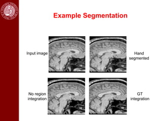
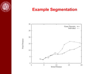
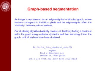
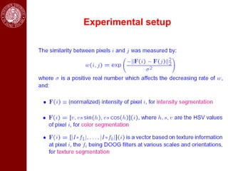
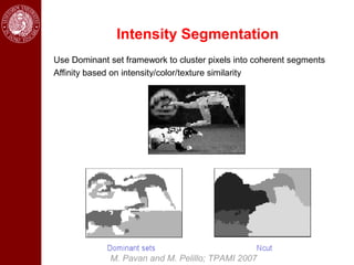
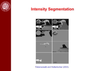
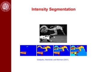
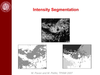
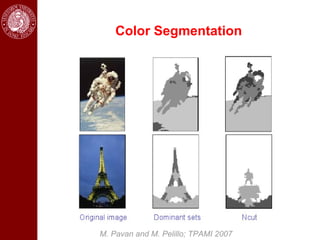
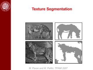
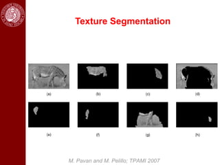
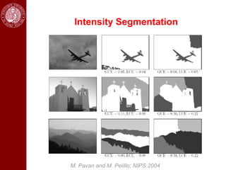
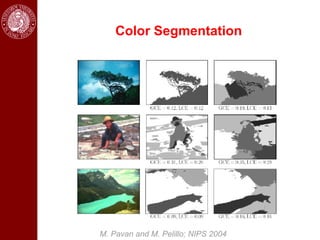
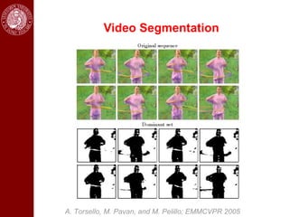
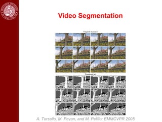
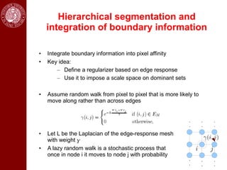
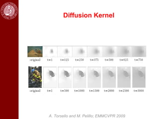
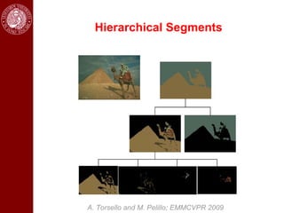
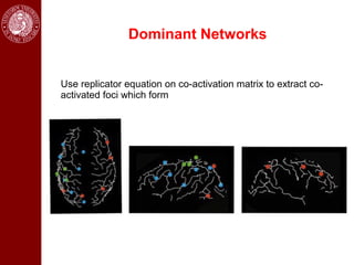
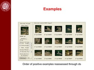
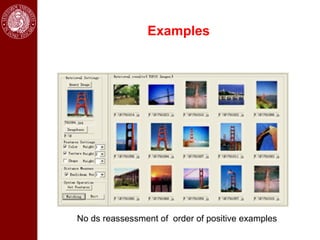
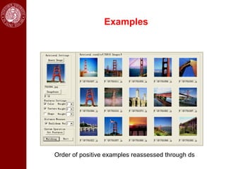
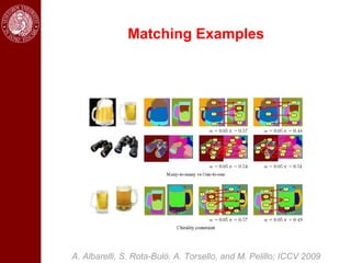
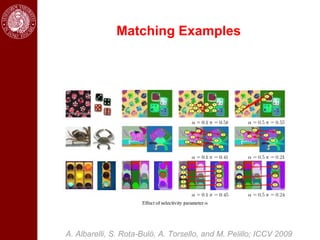
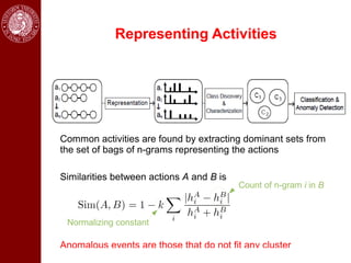
- The document contains a table of contents listing applications of image segmentation, including medical image analysis. - It then discusses using game theory to integrate region-based and boundary-based image segmentation approaches. Pixels and boundaries are modeled as players in a game, with the goal of maximizing both region and boundary posteriors through limited interaction. - Dominant sets, a graph-based clustering technique, is also discussed for applications like intensity, color, texture segmentation of images and video. Hierarchical segmentation is achieved by regularizing dominant sets with boundary information.

1. Table of Content
Applications
– Image Segmentation
– Medical Image Analysis
– Content-Based Image Retrieval
– Matching and Inlier Selection
– Detection of Anomalous Behaviour and Selection of
Discriminative Features
Repeated Games and Online Learning
– Learning in Repeated Games
– Learning with Experts and Regret-Based Learning
– Boosting

2. APPLICATIONS

3. Image Segmentation
Image segmentation problem:
Decompose a given image into
segments, i.e. regions containing
“similar” pixels.
First step in many
computer vision problems
Example: Segments might be regions of the image depicting the
same object.
Semantics Problem: How should we infer objects from segments?

4. Segmentation via Image Labeling
(S. Yu and M. Berthod; CVIU 1995)

5. Markov Random Field Formulation
Model pixel label probability through Markov Random Fields
Probability of a particular labeling L is
where VcLc is the clique potential of L in clique c
Assuming a Gibbs distribution, the posteriory probability is
MAP solution is obtained by maximizing

6. Game-Theoretic Formulation
Use game theory to maximize f(L)
Relaxation scheme in which
• Pixels are players
• Labels are available strategies
Payoff of pixel i depends on the labels of its neighbours
Theorem: L is a local maximum for f(L) iff is it a Nash
equilibrium for the defined game

7. Relaxation Scheme
1. Initialize
2. At iteration k, for each object i, choose a label
If accept the new label with
probability α, otherwise reject it
3. If L( k+1) is a Nash point, stop, else go to step 2
Proposition: for any 0<α<1, L(k) converges to a Nash equilibrium
Note: randomization is necessary to avoid oscillations

8. Relation to Relaxation Labeling
If the potentials of cliques of size greater than 2 sum to zero
the game is a polymatrix game and is thus related to
relaxation labelling
The proposed relaxation scheme thus generalizes (discrete)
relaxation labeling to higher order clique potentials

9. Texture Segmentation

10. Example Segmentation

11. Integration of region and
boundary modules
(A. Chakraborty and J. S. Duncan; TPAMI 1999)

12. Integration of Region and Boundary
Goal is to integrate region-based approaches with boundary-
based approaches
Objectives of region-based and boundary-based are
incommensurable
Due to exponential explosion of pixel dependencies in the
general case, attempts to integrate the approaches into a
single objective function result in ad hoc solutions
Avoid the problem of single-objective by casting it into a game
theoretic framework in which the output of one module affects
the objective function of the other

13. Integration of Region and Boundary
Generalized two player game in which strategies are a
continuum
• The players are the region module and the boundary
module
• The strategies are the possible region and boundary
configurations
The payoff for each player is the posterior of the module
The selection of one module enters as a prior in the
computation of the posterior of the other module
(limited interaction)

14. Region and Boundary Modules
The region is modeled through a Markov Random Field
• Pixels labels x are estimated maximizing the posterior
conditioned to the intensity observations Y and the
boundary prior p
The boundary is modeled through a snake model
• Boundary curve p is estimated maximizing the posterior
conditioned to the gradient observations I and the
boundary prior x

15. Synthetic Example
Input image Region only Boundary only
Region after Boundary after Overlaid on
GT integration GT integration the template

16. Example segmentation
Input image Single function
integration
Game theoretic Overlaid on
integration template

17. Comparison vs. Single Objective

18. Example Segmentation
Input image Hand
segmented
No region GT
integration integration

19. Example Segmentation

20. Example Segmentation
Input image Hand
segmented
No region GT
integration integration

21. Example Segmentation

22. Segmentation Using Dominant Sets

23. Graph-based segmentation
Partition_into_dominant_sets(G)
repeat
find a dominant set
remove it from graph
until all vertices have been clustered

24. Experimental setup

25. Intensity Segmentation
Use Dominant set framework to cluster pixels into coherent segments
Affinity based on intensity/color/texture similarity
M. Pavan and M. Pelillo; TPAMI 2007

26. Intensity Segmentation

27. Intensity Segmentation

28. Intensity Segmentation
M. Pavan and M. Pelillo; TPAMI 2007

29. Color Segmentation
M. Pavan and M. Pelillo; TPAMI 2007

30. Texture Segmentation
M. Pavan and M. Pelillo; TPAMI 2007

31. Texture Segmentation
M. Pavan and M. Pelillo; TPAMI 2007

32. Out-of sample Segmentation
Pairwise clustering has problematic scaling behavior
Subsample the pixels and assigning out-of-sample pixels after
the clustering process has taken place
Can be computed in linear time w.r.t. the size of S

33. Intensity Segmentation
M. Pavan and M. Pelillo; NIPS 2004

34. Color Segmentation
M. Pavan and M. Pelillo; NIPS 2004

35. Alternative Approach
Recall that the probability of a surviving strategy at
equilibrium is related to the centrality of the element to the
cluster
Use the element with higher probability as a class prototype
Assign new elements to the class with the most similar
prototype
Constant time w.r.t. the size of the clusters
Ideal for very large datasets (video)

36. Video Segmentation
A. Torsello, M. Pavan, and M. Pelillo; EMMCVPR 2005

37. Video Segmentation
A. Torsello, M. Pavan, and M. Pelillo; EMMCVPR 2005

38. Hierarchical segmentation and
integration of boundary information
• Integrate boundary information into pixel affinity
• Key idea:
– Define a regularizer based on edge response
– Use it to impose a scale space on dominant sets
• Assume random walk from pixel to pixel that is more likely to
move along rather than across edges
• Let L be the Laplacian of the edge-response mesh
with weight 
• A lazy random walk is a stochastic process that
once in node i it moves to node j with probability

39. Diffusion Kernel
A. Torsello and M. Pelillo; EMMCVPR 2009

40. Regularized Quadratic Program
• Define the regularized quadratic program
• Proposition: Let λ1 (A), λ2 (A), . . . , λn (A) represent the largest,
second largest,..., smallest eigenvalue of matrix A
If then ft is a strictly concave function in Δ.
Further, if the only solution of the regularized
quadratic program belongs to the interior of Δ.

41. Selection of relevant scales
• How do we chose the  at which to separate the levels?
• A good choice should be stable: cohesiveness should not change
much.
• Consider the entropy of the selected cluster
– It is a measure of the size and compactness of the cluster
• Cut on plateaus of the entropy

42. Hierarchical Segments
A. Torsello and M. Pelillo; EMMCVPR 2009

43. Hierarchical Segments
A. Torsello and M. Pelillo; EMMCVPR 2009

44. References
S. Yu and M. Berthod. A Game Strategy Approach for Image Labeling. CVIU 1995.
A. Chakraborty and J. S. Duncan. Game-Theoretic Integration for Image
Segmentation. PAMI 1999.
M. Pavan and M. Pelillo. A new graph-theoretic approach to clustering and
segmentation. CVPR 2003.
M. Pavan and M. Pelillo. Dominant sets and hierarchical clustering. ICCV 2003.
M. Pavan and M. Pelillo. Efficient out-of-sample extension of dominant-set clusters.
NIPS 2004.
A. Torsello, M. Pavan, and M. Pelillo. Spatio-temporal segmentation using dominat
sets. EMMCVPR 2005.
A. Torsello, S. Rota Bulò and M. Pelillo. Grouping wit asymmetric affinities: A game-
theoretic perspective. CVPR 2006.
M. Pavan and M. Pelillo. Dominant sets and pairwise clustering. PAMI 2007.
A. Torsello and M. Pelillo. Hierarchical Pairwise Segmentation Using Dominant Sets
and Anisotropic Diffusion Kernels. EMMCVPR 2009.

45. Medical Image Analysis

46. Analysis of fMRI images
Problems
• detect coherent subregions in cortical areas on the basis of
similarities between fMRI time series
• Localization of activation foci, i.e., functional networks
related to a specific cognitive task

47. Experimental Setup
Patient assigned a word matching Stroop task
This task requires a subject to respond to a particular stimulus
dimension while a competing stimulus dimension has to be
suppressed.
Top row answers: NO
Bottom row answers: YES
Brain response is tracked through time

48. Parcellation
Parcellation is the process of
subdividing a ROI into functional
subregions
Apply replicator equation on the
matrix of correlation of each voxel
time-series
Extract clusters that form
connected and compact
components
Results are consistent with brain
physiology

49. Within-Subject Variability
Inter- and intra-subject variability is low

50. Meta-Analysis:
Recognition of Networks
The reconstruction of functional networks require the analysis
of co-activation of foci
1. Extract foci from activation maxima
2. Computation of co-activation maxima

51. Activated Foci
Activation foci are calculated from the list of activation maxima

52. Dominant Networks
Use replicator equation on co-activation matrix to extract co-
activated foci which form

53. References
G. Lohmann and S. Bohn. Using Replicator Dynamics for Analyzing
fMRI Data of the Human Brain. IEEE Trans on Medical Imaging 2002.
J. Neumann et al. Meta-Analysis of Functional Imaging Data Using
Replicator Dynamics. Human Brain Mapping 2005.
J. Neumann et al. The parcellation of cortical areas using replicator
dynamics in fMRI. Neuroimage 2006.

54. Content-Based Image Retrieval
M. Wang, Z.-L. Ye, Y. Wang, and S.-X. Wang. Dominant sets
clustering for image retrieval. Signal Processing, 2008

55. Content-Based Image Retrieval
Content-based image retrieval focus on searching
images in database similar to the query image
There exists a semantic gap between the limited descriptive
power of low-level visual features and high-level concepts.
Relevance feedback: Use user feedback to improve relevance
of images retrieved from a query image

56. Approach
1. Use feature vector distance 5. Rearrange distances d(g) by
for initial query image descenting order
2. User labels into relevant (I+) 6. Cluster images into similarity
and irrelevant (I-) sets clusters with dominant sets
3. Construct training set (gi,yi) and report in order of
importance within each cluster
7. If further refinement
necessary, repeat steps 2 to 7
4. Train SVM to obtain distance
d(g) between features of Dominant sets are used to
relevant images and classifier reassess relevance order in the
surface positive set (step 6)

57. Approach

58. Examples
No ds reassessment of order of positive examples

59. Examples
Order of positive examples reassessed through ds

60. Examples
No ds reassessment of order of positive examples

61. Examples
Order of positive examples reassessed through ds

62. Precision and Recall

63. Matching and Inlier Selection

64. Matching Problem
The matching problem is one of finding correspondences within a set
of elements, or features
Central to any recognition task where the object to be recognized is
naturally divided into several parts
Correspondences are allowed to compete with one another in a
matching game, a non-cooperative game where
• potential associations between the items to be matched
correspond to strategies
• payoffs reflect the degree of compatibility between competing
hypotheses
The solutions of the matching problem correspond to ESS’s
(dominant sets in the association space)
The framework can deal with general many-to-many matching
problems even in the presence of asymmetric compatibilities.

65. Matching game
Let O1 and O2 be the two sets of features that we want to match and A ⊆
O1 × O2 the set of feasible associations that satisfy the unary constraints.
Each feasible association represents a possible matching hypothesis.
Let C : A × A → R+ be a set of pairwise compatibilities that measure the
support that one association gives to the other.
A submatch (or simply a match) is a set of associations, which satisfies the
pairwise feasibility constraints, and two additional criteria:
– High internal compatibility, i.e. the associations belonging to the match are
mutually highly compatible
– low external compatibility, i.e. associations outside the match are scarcely
compatible with those inside.
.
The proposed approach generalizes the association graph technique
described by Barrow and Burstall to continuous structural constraints

66. Properties of Matching Games
Domain-specific information is confined to the definition of the
compatibility function.
We are able to deal with many-to-many, one-to-many, many-
to-one and one-to-one relations incorporating any hard binary
constraints with the compatibilities (setting them to 0)
Theorem: Consider a matching-game with compatibilities C =
(cij) with cij ≥ 0 and cii = 0. If x ∈ Δ is an ESS then cij > 0 for all i,
j ∈ σ(x)

67. Matching Examples
A. Albarelli, S. Rota-Bulò, A. Torsello, and M. Pelillo; ICCV 2009

68. Matching Examples
A. Albarelli, S. Rota-Bulò, A. Torsello, and M. Pelillo; ICCV 2009

69. GT Matcher and Sparsity
The game-theoretic matcher deviates from the quadratic
assignment tradition in that it is very selective: it limits to
a cohesive set of association even if feasible
associations might still be available
The matcher is tuned towards low false positives rather
than low false negatives such as quadratic assignment
Quadratic assignment is greedy while the game
theoretic matcher favours sparsity in the solutions

70. Matching and Inlier selection
There is a domain in which this property is particularly useful:
Inlier selection
When estimating a transformation acting on some data, we
often need to find correspondences between observations
before and after the transformation
Inlier selection is the process of selecting correspondences
that are consistent with a single global transformation to be
estimated even in the presence of several outlier observations
Examples of problems include surface registration or point-
feature matching

71. Matching and Inlier selection
Typical matching strategies are based on random
selection (RANSAC) or the use of local information such
as feature descriptors.
Global coherence checks are only introduced after a first
estimation (filtering)
Filtering approaches are not very robust w.r.t. outliers
(or structured noise)
The game theoretic approach drives the selection of
correspondences that satisfy a global compatibility
criterion

72. Estimation of Similarity
Transformation
Lowe GT
Input images SIFT features (RANSAC) matcher
A. Albarelli, S. Rota-Bulò, A. Torsello, and M. Pelillo; ICCV 2009

73. Estimation of Similarity
Transformation
A. Albarelli, S. Rota-Bulò, A. Torsello, and M. Pelillo; ICCV 2009

74. Surface Registration
DARCES Spin Images GT matcher
Descriptors are used just to
reduce the set of feasible
associations A
Compatibilities are related to
rigidity constraints
(difference in distances
between corresponding
points)
No initial motion estimation
required (coarse)
A. Albarelli, E.Rodolà, and A. Torsello; CVPR 2010

75. Surface Registration
A. Albarelli, E.Rodolà, and A. Torsello; CVPR 2010

76. Surface Registration
A. Albarelli, E.Rodolà, and A. Torsello; CVPR 2010

77. Point-Matching for Multi-View
Bundle Adjustment
Define (local) compatibility between candidate
correspondences through a weak (affine) camera model
We use the orientation and scale information in the feature
descriptors to infer an affine transformation between the
corresponding features Correspondence imply transformation
Two correspondences are compatible if they define similar
transformations

78. Experiments
A. Albarelli, E.Rodolà, and A. Torsello; 3DPVT 2010

79. Experiments
A. Albarelli, E.Rodolà, and A. Torsello; 3DPVT 2010

80. Experiments
A. Albarelli, E.Rodolà, and A. Torsello; 3DPVT 2010

81. References
A. Albarelli, S. Rota Bulò , A. Torsello, and M. Pelillo. Matching
as a Non-Cooperative Game. ICCV 2009.
A. Albarelli, E. Rodolà, and A. Torsello. Robust Game-
Theoretic Inlier Selection for Bundle Adjustment. 3DPVT 2010.
A. Albarelli, E. Rodolà, and A. Torsello. A Game-Theoretic
Approach to Fine Surface Registration without Initial Motion
Estimation. CVPR 2010.
A. Albarelli, E. Rodolà, and A. Torsello. Imposing Semi-local
Geometric Constraints for Accurate Correspondences
Selection in Structure from Motion: a Game-Theoretic
Perspective. IJCV 2011.

82. Detection of Anomalous Behaviour
and
Selection of Discriminative Features

83. Representing Activities
Represents human activities as
sequence of atomic actions
Divide sequences into fixed length
pieces (n-grams)
Represent full actions as a bag of
n-grams
R. Hamid et al. Artificial Intelligence 2009

84. Representing Activities
Common activities are found by extracting dominant sets from
the set of bags of n-grams representing the actions
Similarities between actions A and B is
Count of n-gram i in B
Normalizing constant
Anomalous events are those that do not fit any cluster

85. Deciding the (Ab)Normality
Decide the (ab)normality of a new instance based on its
closeness to the members of the closest activity-class
This is done with respect to the average closeness between
all the members of the class
A new action i is regular wrt the closest class S if ,
where T is learned from the training set

86. Example Activity Classification
R. Hamid et al. Artificial Intelligence 2009

87. Example Anomalous Activity
R. Hamid et al. Artificial Intelligence 2009

88. Selection of Discriminative Features
Adopt a similar approach to the selection of discriminative
features among a large number of highly similar features
Extract clusters of similar features and iteratively throw them
away, leaving only uncommon and discriminative features
Uses the fact that dominant set is not a partitioning scheme,
but an unsupervised one-class classifier

89. Application to Surface Registration
A. Albarelli, E.Rodolà, and A. Torsello; ECCV 2010

90. Application to Surface Registration
A. Albarelli, E.Rodolà, and A. Torsello; ECCV 2010

91. Recognition with Textured
Background
A. Albarelli, E.Rodolà, and A. Torsello; ICPR 2010

92. Recognition with Textured
Background
A. Albarelli, E.Rodolà, and A. Torsello; ICPR 2010

93. References
R. Hamid et al. Detection and Explanation of Anomalous Activities:
Representing Activities as Bags of Event n-Grams. CVPR 2005.
R. Hamid et al. A Novel Sequence Representation for Unsupervised
Analysis of Human Activities. Artificial Intelligence 2009.
A. Albarelli, E. Rodolà, and A. Torsello. Loosely Distinctive Features
for Robust Surface Alignment. To appear ECCV 2010.
A. Albarelli, E. Rodolà, A. Cavallarin, and A. Torsello. Robust Figure
Extraction on Textured Background: a Game-Theoretic Approach. To
appear ICPR 2010.

94. Repeated Games and
Online Learning

95. Repeated Games
Previous assumptions:
– players had complete knowledge of the game
– the game was played only once
What happens if the payoffs are not known, but the game
can be repeated?
Can a player learn a good strategy from the past plays?

96. Repeated Games
Previous approach:
– just compute an optimal/equilibrium strategy
Another approach:
– learn how to play a game by playing it many times,
and updating your strategy based on experience
Why?
– Some of the game’s utilities (especially the other
players’) may be unknown to you
– The other players may not be playing an
equilibrium strategy
– Computing an optimal strategy can be hard
– Learning is what humans typically do

97. Iterated Prisoner's Dilemma
Prisoner's dilemma
Player 1
defect cooperate
defect -10,-10 -1,-25
Player 2
cooperate -25,-1 -3,-3
What strategies should one apply?
Can I adapt to a player willing to cooperate and cooperate myself?
Although the Prisoner's dilemma has only one Nash equilibrium
(everyone defect), cooperation can be sustained in the repeated
Prisoner's dilemma if the players are interested enough in future
outcomes of the game to take some loss in early plays.

98. Tit for Tat
It was first introduced by Anatol Rapoport in Robert Axelrod's two
tournaments, held around 1980.
Although extremely simple it won both
An agent using this strategy will initially cooperate, then respond in
kind to an opponent's previous action: If the opponent previously was
cooperative, the agent is cooperative. If not, the agent is not.
Properties
1. Unless provoked, the agent will always cooperate
2. If provoked, the agent will retaliate
3. The agent is quick to forgive
4. The agent must have a good chance of competing against the
opponent more than once.
Note: used by BitTorrent to optimize download speed.
(optimistic chocking)

99. Fictitious Play
One widely used model of learning is the process of fictitious play and its
variants.(G.W. Brown 1951).
In it, each player presumes that her/his opponents are playing stationary
(possibly mixed) strategies.
In this process, agents behave as if they think they are facing an unknown
but stationary (possibly mixed) distribution of opponents strategies
The players choose their actions in each period to maximize that period’s
expected payoff given their assessment of the distribution of opponent’s
actions.
The assessment is based on the observed frequencies of the other
players past strategies.
At each round, each player thus best responds to the empirical frequency
of play of his opponent.

100. Convergence of Fictitious Play
Such a method is of course adequate if the opponent indeed
uses a stationary strategy, while it is flawed if the opponent's
strategy is non stationary. The opponent's strategy may for
example be conditioned on the fictitious player's last move.
One key question about fictitious play is whether or not
this play converges
– if it does,then the stationarity assumption employed by
players makes sense, at least asymptotically
– if it does not, then it seems implausible that players will
maintain that assumption

101. Convergence of Fictitious Play
Convergence properties of Fictitious Play
• If s is a strict Nash equilibrium, and s is played at time t in the
process of fictitious play, s is played at all subsequent times.
(strict Nash equilibria are absorbing)
• Any pure strategy steady state of fictitious play must be a Nash
equilibrium
• If the empirical distributions over each player's choices
converge, the strategy profile corresponding to the product of
these distributions is a Nash equilibrium
• The empirical distributions converge if the game is zero-sum
(Miyasawa 1961) or solvable by iterated strict dominance
(Nachbar, 1990)

102. Convergence of Fictitious Play
Fictitious play might not converge (Shapley 1964)
Modified Rock-Scissors-Paper
Player 1
Rock Scissors Paper
Rock 0,0 1,0 0,1
Player 2 Scissors 0,1 0,0 1,0
Paper 1,0 0,1 0,0
if the players start by choosing (Rock, Scissors), the play will
cycle indefinitely.

103. Sequential Prediction
In a sequential prediction problem a predictor (or
forecaster) observes a sequence of symbols
each time t = 1, 2, . . . , before the tth symbol of the
sequence is revealed, the forecaster guesses its value st on
the basis of the previous t−1 observations.
GOAL: limit the number of prediction mistakes without
making any statistical assumptions on the way the data
sequence is generated

104. Stationary Stochastic Process
In the classical statistical learning theory, the sequence of
outcomes, is assumed to be a realization of a
stationary stochastic process
Statistical properties of the process, and effective prediction
rules are estimated on the basis of past observations
In such a setup, the risk of a prediction rule may be defined
as the expected value of some loss function
Different rules are compared based on their risk.

105. Game against the Environment
We want to abandon the idea of a stationary
stochastic process in favor of an unknown (even
adversarial) mechanism
The forecaster plays a game against the
environment, which can, in principle, respond to the
forecaster's previous predictions
The goal of the forecaster is to maximize the payoff
associated with his predictions
The goal of the environment is to minimize the
forecaster's payoff

106. Learning with Experts
Without a probabilistic model,
the notion of risk cannot be
defined
There is no obvious baseline
against which to measure the
forecaster’s performance
We provide such baseline
by introducing
reference forecasters,
also called experts.

107. Experts
At time t experts provide an advice in the form of a vector
of predicted symbols
Think of experts as classifiers, observing the environment
and giving a prediction
Experts are not perfect (each expert can be wrong on any
observation)
We want to get good prediction (high payoff) based on
expert advice
A good prediction is consistent with the performance of the
best experts

108. Game against the Environment
The forecaster does not have
• knowledge of the game (payoff function)
• knowledge of the environment's strategy profile
The forecaster knows the payoffs received by each
strategy against each previous play of the environment
However the knowledge is based on the actual pure
strategies selected by the environment, not its strategy
profile

109. Prediction Game
The game is played repeatedly in a sequence of rounds.
1. The environment chooses mixed strategy yt',and plays
(pure) strategy yt according to the distribution yt'
2. The experts provide their predictions
3. The forecaster chooses an expert according to mixed
strategy xt
The forecaster is permitted to observe the payoff
that is, the payoff it would have obtained had it
played following pure strategy (expert) i

110. Prediction Game
The goal of the forecaster is to do almost as well as the best
expert against the actual sequence of plays
That is, the cumulative payoff
Should not be “much worse” that the best (mixed) expert in
hindsight

111. Learnability
There are two main questions regarding this prediction
game
1. Is there a solution? I.e., is there a strategy that will
work even in this adversarial environment?
2. Can we learn such solution based on the previous
plays?

112. Minimax and Learnability
The environment's goal
is to minimize the Zero-sum two player game
forecaster's payoff
We are within the hypotheses of the Minimax theorem
There exists a strategy x such that
The value v is the best the forecaster can be guaranteed
since there exists a strategy y such that
Moreover, (x,y) is a Nash equilibrium

113. Regret
We define the external regret of having played strategy
sequence x=(x1,...,xT) w.r.t. expert e as the loss in payoff we
incurred in by not having followed e's advice
The learner's goal is to minimize the maximum regret w.r.t.
any expert

114. Minimax and Learnability
If the forecaster predicts according to a Nash equilibrium x, he
is guaranteed a payoff v even against and adversarial
environment
Theorem: Let G be a zero-sum game with value v. If the
forecaster plays for T steps a procedure with external regret
R, then its average payoff is at least v-R/T
Algorithm can thus seek to minimize the external regret

115. Regret-Based Learning
Assume {0,1} utilities, and let consider loss L(x,y)=1-u(x,y)
rather than utility u(x,y)
Greedy algorithm
The greedy algorithm at each time t selects the (mixed)
strategy x that, if played for the first t-1 plays, would have
given the minimum regret
The greedy algorithm's loss is
where Lmin is the loss incurred by the best expert
No deterministic algorithm can obtain a better ratio than N!

116. Weighted Majority Forecaster
The idea is to assign weights wi to expert i that reflect its past
performance, and pick an expert with probability proportional to
its weight
Randomized Weighted Majority (RWM) Algorithm
Initially: wi =1 and pi =1/N, for i=1,...,n.
At time t: If Lt= 1 let wt = wt−1(1 − η); else wt = wt-1
Use mixed profile
Randomized Weighted Majority achieves loss

117. Experts and Boosting
In general experts can be any (weak) predictor/classifier
Finding an optimal strategy over expert advices is equivalent
to finding an optimal combination of classifiers
Boosting is the problem of converting a weak learning
algorithm that performs just slightly better than random
guessing into one that performs with arbitrarily good
accuracy
Boosting works by running the weak learning algorithm
many times on many distributions, and to combine the
selected hypotheses into a final hypothesis

118. Boosting
(Y. Freund and R. E. Schapire, 1996)
Boosting proceeds in rounds alternating
1. The booster constructs a distribution p(k) on the
sample space X and passes it to the weak learner
2. The weak learner produces an hypothesis h(k) ∈ H with
error at most ½ - ;
After T rounds the hypotheses h(1),...,h(T) are combined into a
final hypothesis h
Main questions
– How do we chose p(k)?
– How do we combine the hypotheses?

119. Boosting and Games
Define a two player game where
– the booster's strategies are related to the possible samples
– the weak learner's strategies are the available hypotheses
– The booster's payoff is defined as follows:
target concept
The boosters's goal is to feed a bad distributions to the weak learner
Due to the minimax theorem we have
Less than half of the hypotheses are wrong!
Combine them by weighted majority (weighted according to h*)

120. Boosting and Games
Alternate the game
1. The weak learner returns a guaranteed optimal
hypothesis ht satisfying
2. The booster responds by using randomized weighted
majority approach to compute distribution pt* over
samples
After T repetitions, the boosted hypothesis h* on a new
sample x is obtained by majority voting among h1(x),...,hT(x)

121. References
Y. Freund and R. E. Schapire. Game Theory, On-line Prediction and
Boosting. COLT 1996.
D. Fudenberg and D. K. Levine. The Theory of Learning in Games.
The MIT Press, 1998.
N. Cesa-Bianchi and G. Lugosi. Prediction, Learning, and Games.
Cambridge University Press, 2006.
A. Blum and Y. Mansour. Chapter 4 “Learning, Regret minimization,
and Equilibria” in N. Nisan, T. Roughgarden, E. Tardos, and V.
Vazirani (Eds.), Algorithmic Game Theory, 2007.