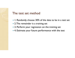
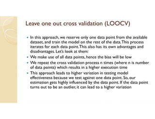
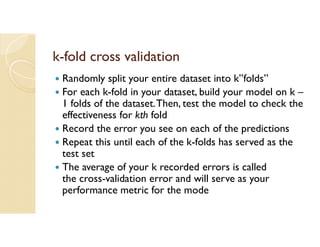
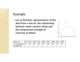
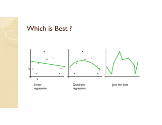
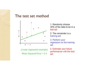
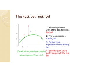
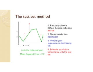
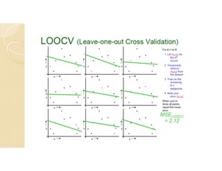
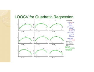
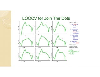
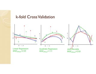
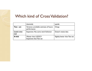
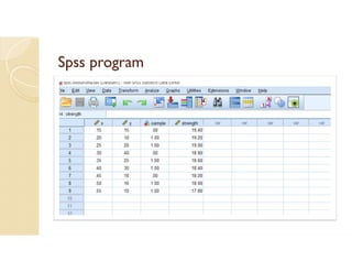
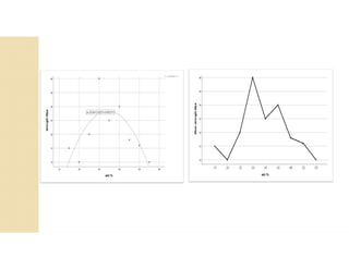
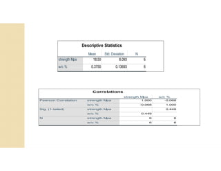
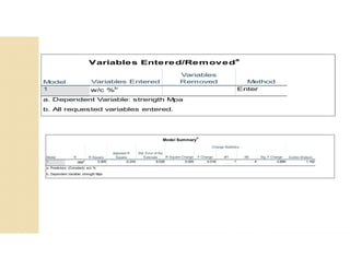
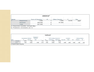
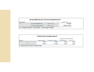
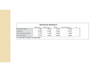
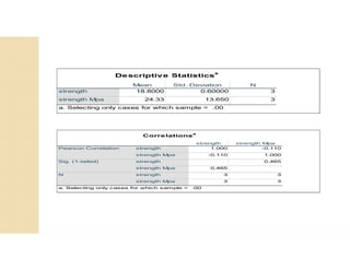
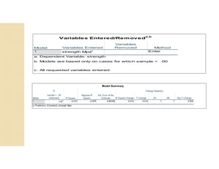
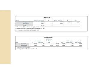
Cross-validation is a technique used to evaluate machine learning models by reserving a portion of a dataset to test the model trained on the remaining data. There are several common cross-validation methods, including the test set method (reserving 30% of data for testing), leave-one-out cross-validation (training on all data points except one, then testing on the left out point), and k-fold cross-validation (randomly splitting data into k groups, with k-1 used for training and the remaining group for testing). The document provides an example comparing linear regression, quadratic regression, and point-to-point connection on a concrete strength dataset using k-fold cross-validation. SPSS output for the

1. CrossValidation
By
AbdulRidha Mohammad

2. content layout
 Introduction
 Methods of CrossValidation
Test set method
Leave one out cross validation (LOOCV)
k-fold cross validation
 Example
 Spss programing

3. What is CrossValidation?
 CrossValidation is a technique which involves reserving a
particular sample of a dataset on which you do not train the
model. Later, you test your model on this sample before
finalizing it.
 Here are the steps involved in cross validation:
 You reserve a sample data set
 Train the model using the remaining part of the dataset
 Use the reserve sample of the test (validation) set.This will
help you in gauging the effectiveness of your model’s
performance. If your model delivers a positive result on
validation data, go ahead with the current model. It rocks!

4. Methods of CrossValidation
 A few common methods used for CrossValidation
There are various methods available for performing cross
validation. I’ve discussed a few of them in this section.
 The test set method
 Leave one out cross validation (LOOCV)
 k-fold cross validation

5. The test set method
 1. Randomly choose 30% of the data to be in a test set
 2.The remainder is a training set
 3. Perform your regression on the training set
 4. Estimate your future performance with the test

6. Leave one out cross validation (LOOCV)
 In this approach, we reserve only one data point from the available
dataset, and train the model on the rest of the data.This process
iterates for each data point.This also has its own advantages and
disadvantages. Let’s look at them:
 We make use of all data points, hence the bias will be low
 We repeat the cross validation process n times (where n is number
of data points) which results in a higher execution time
 This approach leads to higher variation in testing model
effectiveness because we test against one data point. So, our
estimation gets highly influenced by the data point. If the data point
turns out to be an outlier, it can lead to a higher variation

7. k-fold cross validation
 Randomly split your entire dataset into k”folds”
 For each k-fold in your dataset, build your model on k –
1 folds of the dataset.Then, test the model to check the
effectiveness for kth fold
 Record the error you see on each of the predictions
 Repeat this until each of the k-folds has served as the
test set
 The average of your k recorded errors is called
the cross-validation error and will serve as your
performance metric for the mode

8. Example
 Let us find best representation of the
data from a test for the relationship
between water cement ration and
the compressive strength of
concrete as below:
X=w/c % 0.15 0.2 0.25 0.3 0.35 0.4 0.45 0.5 0.55
Y=Compressive
strength Mpa
15 10 20 40 25 30 18 16 10

9. Which is Best ?
Linear
regression
Quadratic
regression
Join the dots

10. The test set method

11. The test set method

12. The test set method

16. k-fold CrossValidation
 Randomly break the dataset into k partitions (in our
example we’ll have k=3 partitions colored Red Green
and Blue).
 For every partition:Train on all the points not in the
same partition.
 Find the test-set sum of errors on the taken points.
 Then report the mean error

17. k-fold CrossValidation

18. Which kind of CrossValidation?
downside upside
Test - set Variance: unreliable estimate of future
performance
Cheap
Leave one-
out
Expensive. Has some weird behavior Doesn’t waste data
K-fold Waster than LOOCV
Expensive thanTest set
Slightly better than Test set

19. Spss program

22. Mean Std. Deviation N
strength Mpa 18.50 8.093 6
w/c % 0.3750 0.13693 6
Descriptive Statistics
strength Mpa w/c %
strength Mpa 1.000 -0.068
w/c % -0.068 1.000
strength Mpa 0.449
w/c % 0.449
strength Mpa 6 6
w/c % 6 6
Correlations
Pearson Correlation
Sig. (1-tailed)
N

23. Variables Entered
Variables
Removed Method
1 w/c %b Enter
Variables Entered/Removed
a
Model
a. Dependent Variable: strength Mpa
b. All requested variables entered.
R Square Change F Change df1 df2 Sig. F Change
1 .068
a 0.005 -0.244 9.028 0.005 0.018 1 4 0.899 1.162
a. Predictors: (Constant), w/c %
b. Dependent Variable: strength Mpa
Model Summary
b
Model R R Square
Adjusted R
Square
Std. Error of the
Estimate
Change Statistics
Durbin-Watson

24. Sum of Squares df Mean Square F Sig.
Regression 1.500 1 1.500 0.018 .899
b
Residual 326.000 4 81.500
Total 327.500 5
ANOVA
a
Model
1
a. Dependent Variable: strength Mpa
b. Predictors: (Constant), w/c %
Standardized
Coefficients
B Std. Error Beta Lower Bound Upper Bound Zero-order Partial Part Tolerance VIF
(Constant) 20.000 11.655 1.716 0.161 -12.359 52.359
w/c % -4.000 29.484 -0.068 -0.136 0.899 -85.862 77.862 -0.068 -0.068 -0.068 1.000 1.000
1
a. Dependent Variable: strength Mpa
Coefficients
a
Model
Unstandardized Coefficients
t Sig.
95.0% Confidence Interval for B Correlations Collinearity Statistics

25. w/c %
Correlations w/c % 1.000
Covariances w/c % 869.333
Coefficient Correlations
a
Model
1
a. Dependent Variable: strength Mpa
(Constant) w/c %
1 1.949 1.000 0.03 0.03
2 0.051 6.162 0.97 0.97
a. Dependent Variable: strength Mpa
Collinearity Diagnostics
a
Model Eigenvalue Condition Index
Variance Proportions
1

26. Minimum Maximum Mean Std. Deviation N
Predicted Value 17.80 19.20 18.50 0.548 6
Residual -9.200 11.600 0.000 8.075 6
Std. Predicted Value -1.278 1.278 0.000 1.000 6
Std. Residual -1.019 1.285 0.000 0.894 6
Residuals Statistics
a
a. Dependent Variable: strength Mpa

27. Mean Std. Deviation N
strength 18.8000 0.60000 3
strength Mpa 24.33 13.650 3
Descriptive Statistics
a
a. Selecting only cases for which sample = .00
strength strength Mpa
strength 1.000 -0.110
strength Mpa -0.110 1.000
strength 0.465
strength Mpa 0.465
strength 3 3
strength Mpa 3 3
Correlations
a
Pearson Correlation
Sig. (1-tailed)
N
a. Selecting only cases for which sample = .00

28. Variables Entered
Variables
Removed Method
1 strength Mpac Enter
Variables Entered/Removed
a,b
Model
a. Dependent Variable: strength
b. Models are based only on cases for which sample = .00
c. All requested variables entered.
R
sample = .00
(Selected) R Square Change F Change df1 df2 Sig. F Change
1 .110a 0.012 -0.976 0.84339 0.012 0.012 1 1 0.930
a. Predictors: (Constant), strength Mpa
Model Summary
Model R Square
Adjusted R
Square
Std. Error of the
Estimate
Change Statistics

29. Sum of Squares df Mean Square F Sig.
Regression 0.009 1 0.009 0.012 .930
c
Residual 0.711 1 0.711
Total 0.720 2
ANOVA
a,b
Model
1
a. Dependent Variable: strength
b. Selecting only cases for which sample = .00
c. Predictors: (Constant), strength Mpa
Standardized
Coefficients
B Std. Error Beta Lower Bound Upper Bound
(Constant) 18.918 1.169 16.179 0.039 4.060 33.775
strength Mpa -0.005 0.044 -0.110 -0.111 0.930 -0.560 0.550
1
a. Dependent Variable: strength
b. Selecting only cases for which sample = .00
Coefficients
a,b
Model
Unstandardized Coefficients
t Sig.
95.0% Confidence Interval for B