Downloaded 27 times

![rs = 1 – 6[∑D² + 1/12 (m³ - m) + 1/12 (m³ - m) +.....]
n³ - n
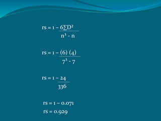
rs = 1 – 6[84 + 1/12 (2³-2) + 1/12 (3³-3) + 1/12 (2³-2) + 1/12 (2³-2)
10³ - 10
rs = 1 – 6[84 + 6/12 + 24/12 + 6/12 + 6/12]
990
rs = 1 – 6[84 + 0.5 + 2 + 0.5 + 0.5]
990
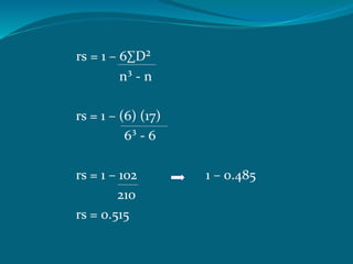
rs = 1 – 525
990
rs = 0.47](https://image.slidesharecdn.com/correlationanalysis-160929134614/85/Correlation-analysis-17-320.jpg)
![r = ±√ ±[2C – n]
√ n
r = ±√±[ (2) (6) – (7)]
√ 7
r = ±√± 0.714
r = 0.845](https://image.slidesharecdn.com/correlationanalysis-160929134614/85/Correlation-analysis-19-320.jpg)


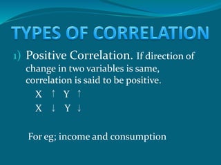
The document discusses correlation as a statistical method to analyze the relationship between variables, detailing positive and negative correlations as well as their degrees. It includes various methods for calculating correlation, such as the scatter diagram and rank methods, along with practical examples and calculations for different datasets. Additionally, it outlines the significance of correlation coefficients in understanding the extent of relationships between variables.


![7.__Developing_a_Research_Proposal[1].pptx](https://cdn.slidesharecdn.com/ss_thumbnails/7-260131073037-df92dd7d-thumbnail.jpg?width=640&height=640&fit=bounds)

![Hacking-Uncovered-How-People-Get-Hacked-and-How-to-Stay-Safe[1].pptx](https://cdn.slidesharecdn.com/ss_thumbnails/hacking-uncovered-how-people-get-hacked-and-how-to-stay-safe1-260130170011-4883a9c7-thumbnail.jpg?width=640&height=640&fit=bounds)


