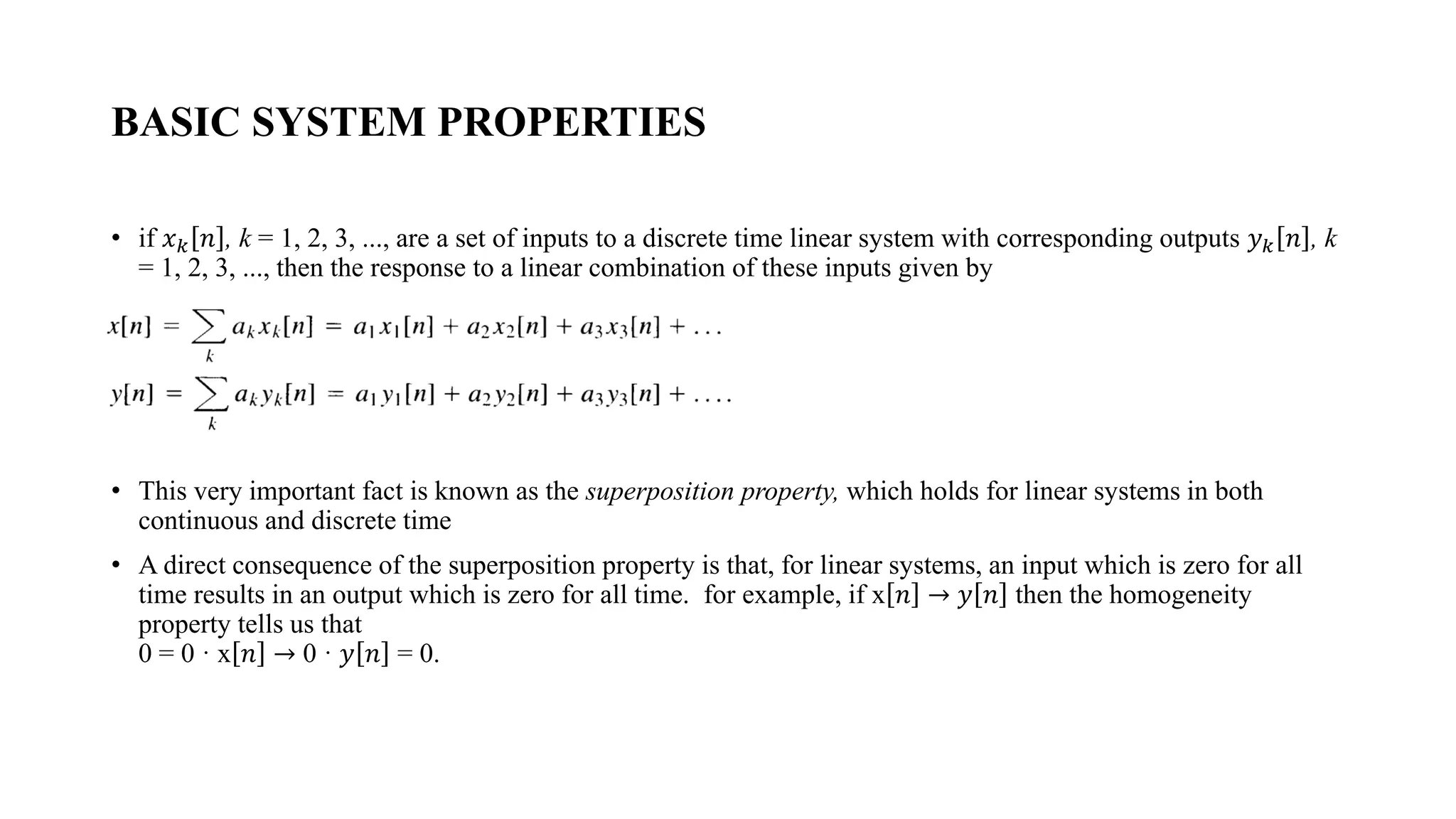
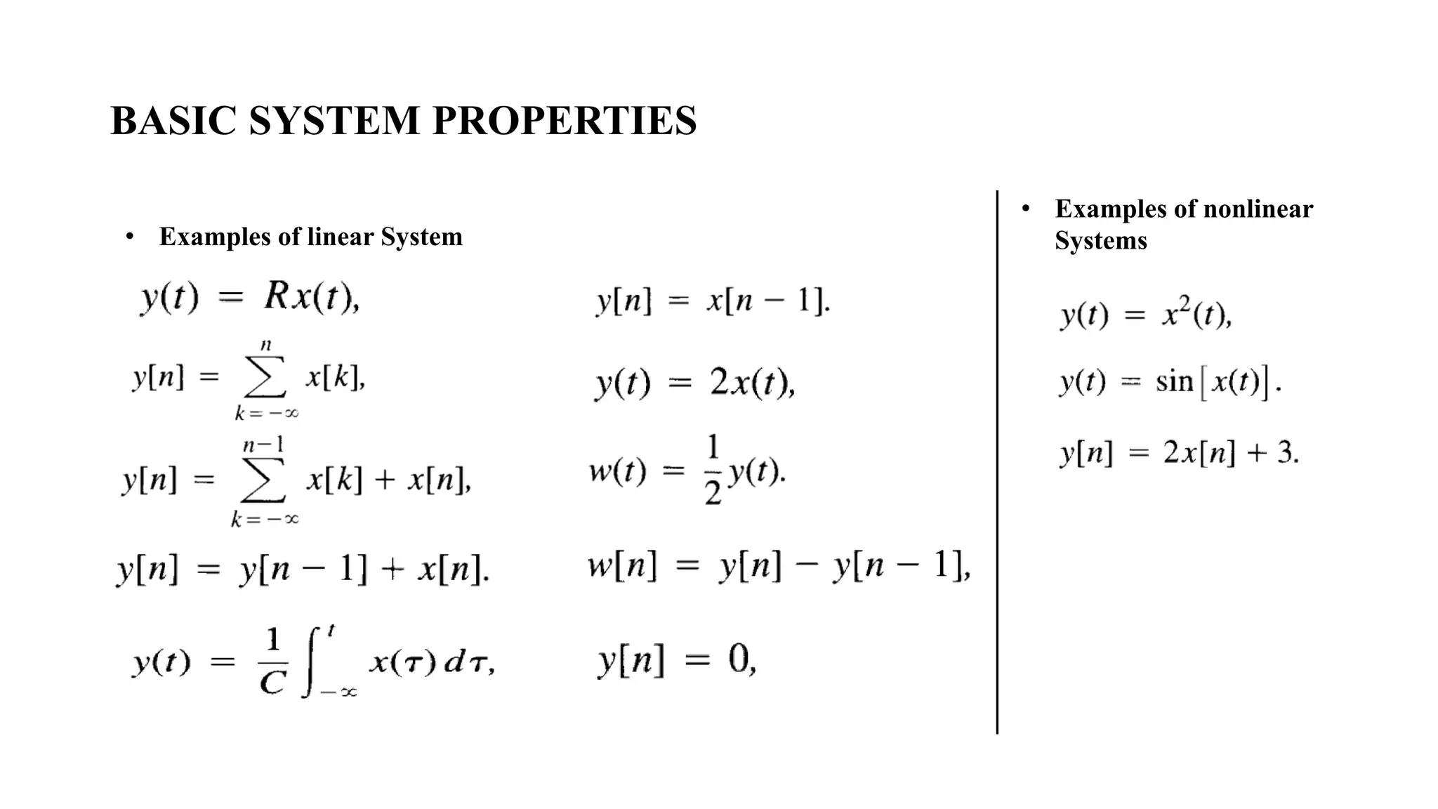
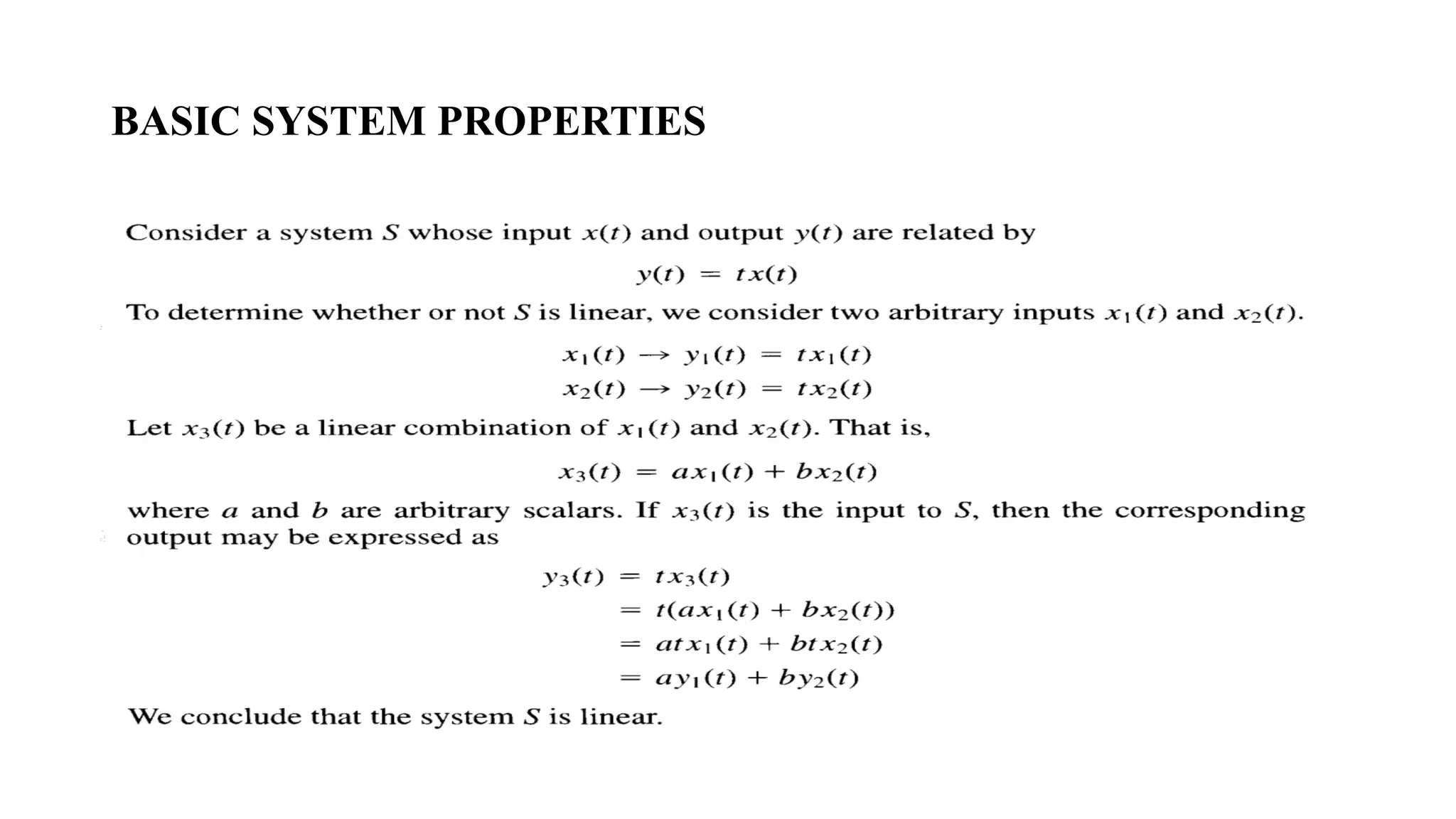
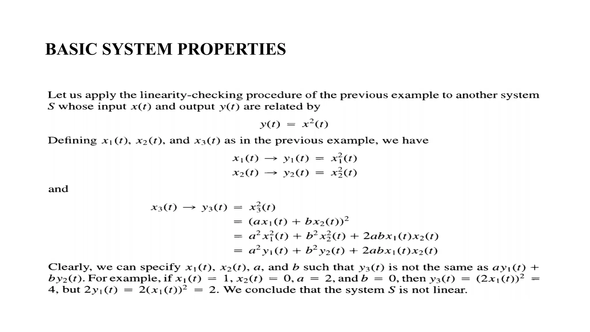
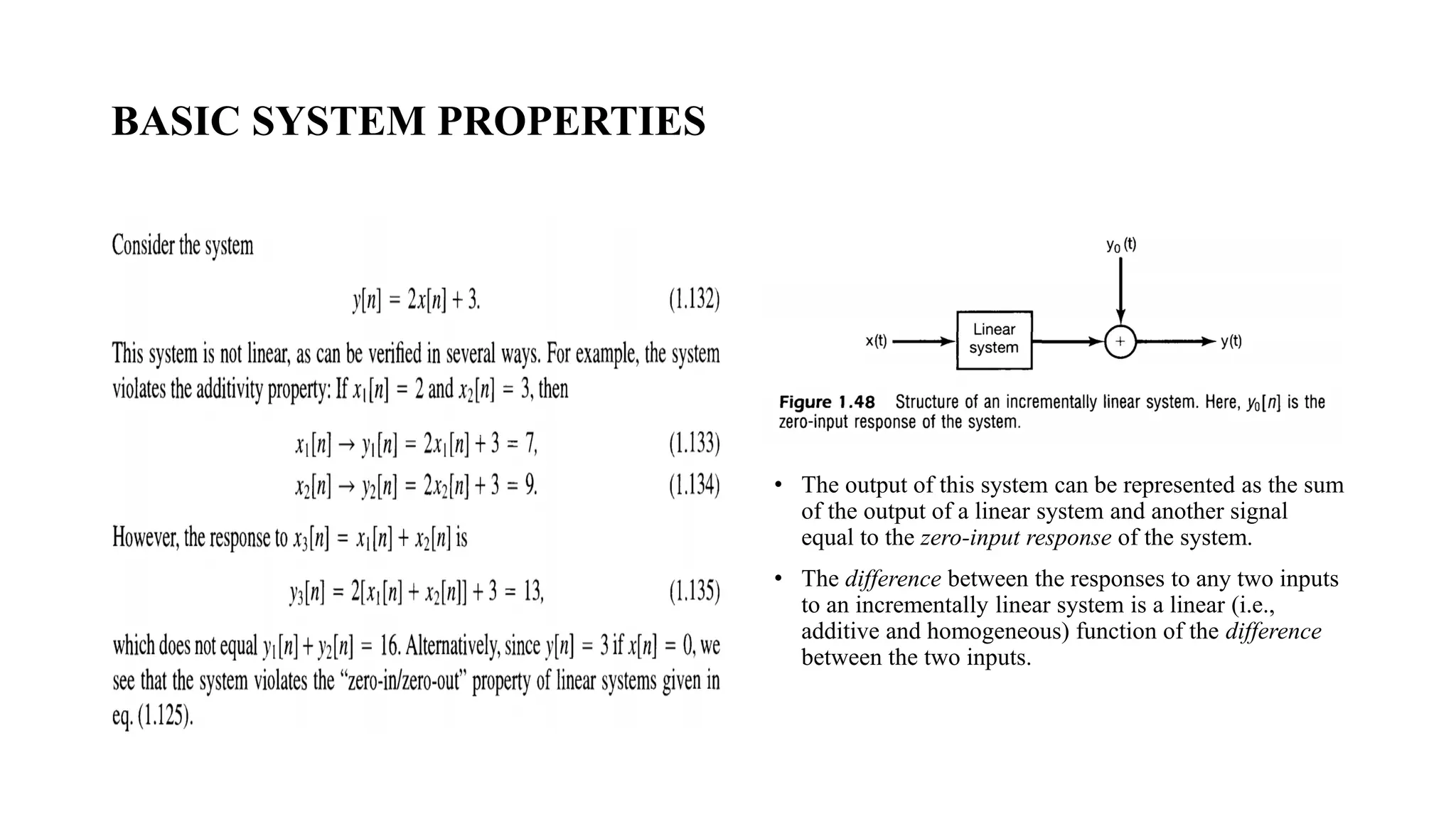
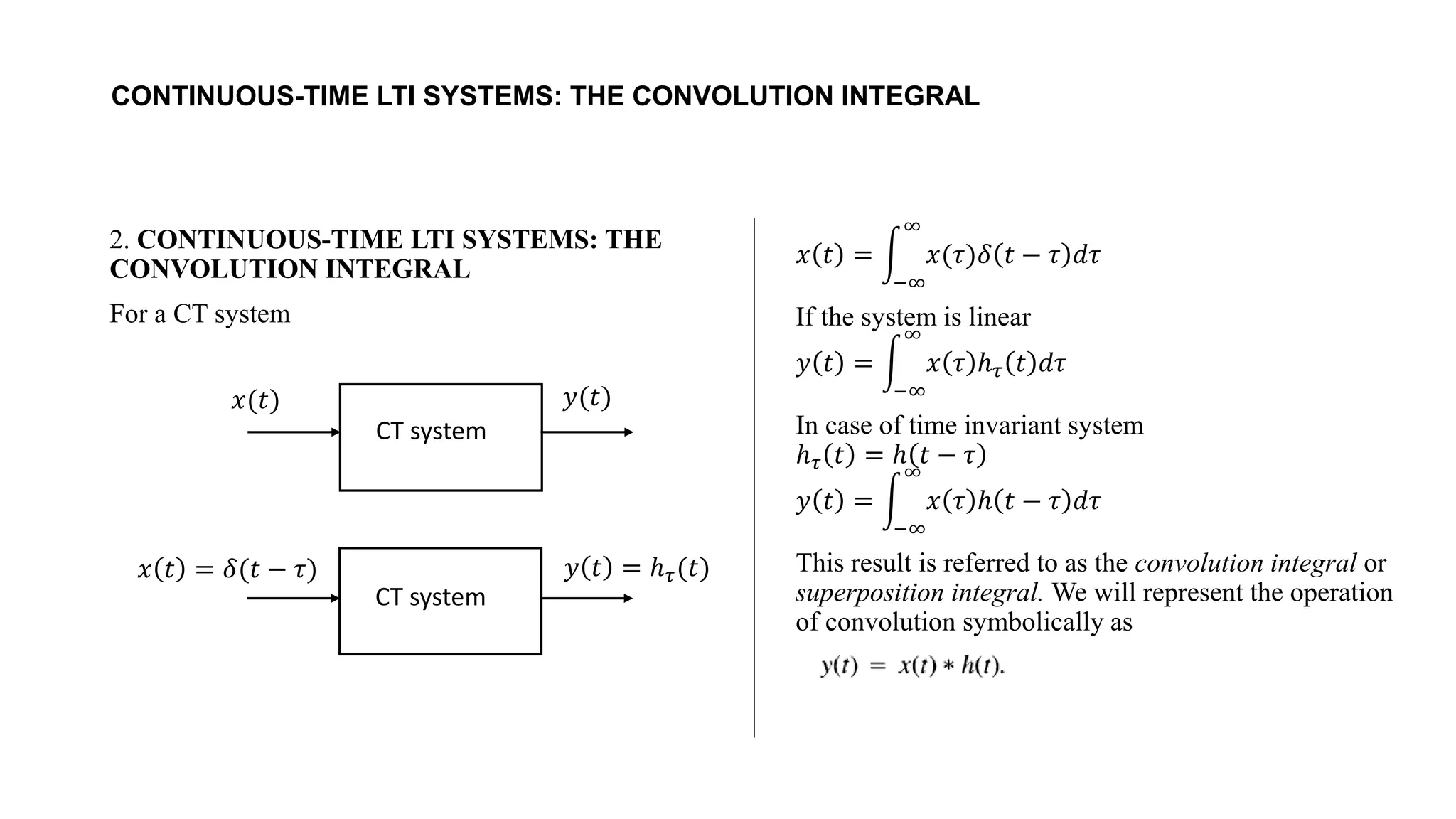
- Linear systems have the properties of additivity and homogeneity, meaning the output is the sum of the individual outputs in response to each input, and scaling the input scales the output accordingly. - For both discrete-time and continuous-time linear time-invariant (LTI) systems, the output can be expressed as the convolution of the input signal and the impulse response of the system. - The convolution represents the superposition of scaled and delayed versions of the impulse response that combine to form the output signal. This convolution representation fully characterizes the behavior of an LTI system.

1. Signal and Systems
Chapter 2
Islam K. Sharawneh
islam.Sharawneh@ptuk.edu.ps

2. BASIC SYSTEM PROPERTIES
6. Linearity
A linear system, in continuous time or discrete time, is a system that possesses the important property of
superposition: If an input consists of the weighted sum of several signals, then the output is the superposition-
that is, the weighted sum-of the responses of the system to each of those signals.
More precisely, let 𝑦1 𝑡 be the response of a continuous time system to an input 𝑥1 𝑡 , and let 𝑦2(𝑡) be the
output corresponding to the input 𝑥2 𝑡 . Then the system is linear if:
1. The response to 𝑥1 𝑡 + 𝑥2 𝑡 is 𝑦1 𝑡 + 𝑦2(𝑡).(additivity property )
2. The response to 𝑎𝑥1 𝑡 is 𝑎𝑦1 𝑡 , where a is any complex constant. (homogeneity property)
The two properties defining a linear system can be combined into a single statement:
𝑎 and 𝑏 are any complex constants.

3. BASIC SYSTEM PROPERTIES
• if 𝑥𝑘 𝑛 , k = 1, 2, 3, ..., are a set of inputs to a discrete time linear system with corresponding outputs 𝑦𝑘 𝑛 , k
= 1, 2, 3, ..., then the response to a linear combination of these inputs given by
• This very important fact is known as the superposition property, which holds for linear systems in both
continuous and discrete time
• A direct consequence of the superposition property is that, for linear systems, an input which is zero for all
time results in an output which is zero for all time. for example, if x 𝑛 → 𝑦 𝑛 then the homogeneity
property tells us that
0 = 0 · x 𝑛 → 0 · 𝑦 𝑛 = 0.

4. BASIC SYSTEM PROPERTIES
• Examples of linear System
• Examples of nonlinear
Systems

5. BASIC SYSTEM PROPERTIES
• Example :
𝑦 𝑡 = ෍
𝑛=−∞
∞
𝑥(𝑡)𝛿(𝑡 − 𝑛𝑇)
Let 𝑥1 𝑡 → 𝑦1 𝑡 𝑎𝑛𝑑 𝑥2 𝑡 → 𝑦2 𝑡
𝑥 𝑡 = 𝛼𝑥1 𝑡
𝑦 𝑡 = ෍
𝑛=−∞
∞
𝑥 𝑡 𝛿 𝑡 − 𝑛𝑇
= σ𝑛=−∞
∞
𝛼𝑥1 𝑡 𝛿 𝑡 − 𝑛𝑇 = 𝛼𝑦1 𝑡
(homogeneous)
𝑥 𝑡 = 𝑥1 𝑡 + 𝑥2(𝑡)
𝑦 𝑡 = ෍
𝑛=−∞
∞
𝑥 𝑡 𝛿 𝑡 − 𝑛𝑇
= ෍
𝑛=−∞
∞
[𝑥1 𝑡 + 𝑥2(𝑡)] 𝛿 𝑡 − 𝑛𝑇
= ෍
𝑛=−∞
∞
𝑥1 𝑡 𝛿 𝑡 − 𝑛𝑇 + ෍
𝑛=−∞
∞
𝑥2 𝑡 𝛿 𝑡 − 𝑛𝑇
= 𝑦1 𝑡 + 𝑦2(𝑡)
(additive)
The system is linear

6. BASIC SYSTEM PROPERTIES

7. BASIC SYSTEM PROPERTIES

8. BASIC SYSTEM PROPERTIES
• The output of this system can be represented as the sum
of the output of a linear system and another signal
equal to the zero-input response of the system.
• The difference between the responses to any two inputs
to an incrementally linear system is a linear (i.e.,
additive and homogeneous) function of the difference
between the two inputs.

9. BASIC SYSTEM PROPERTIES
• Show that the following system is additive but not homogeneous
• Show that the difference between the responses to any two inputs to an
incrementally linear system stated below is a linear (i.e., additive and
homogeneous) function of the difference between the two inputs.

10. LINEAR TIME-INVARIANT SYSTEMS
1. DISCRETE-TIME LTI SYSTEMS: THE CONVOLUTION SUM
The key idea in visualizing how the discrete-time unit impulse can be used to construct any discrete-time signal
is to think of a discrete-time signal as a sequence of individual impulses.
Therefore, the sum of the five sequences in the figure equals x 𝑛 for -2≥ 𝑛 ≥ 2. More generally, by including
additional shifted, scaled impulses, we can write
Writing this summation in a more compact form, we have
(sifting property of the discrete-time unit impulse)

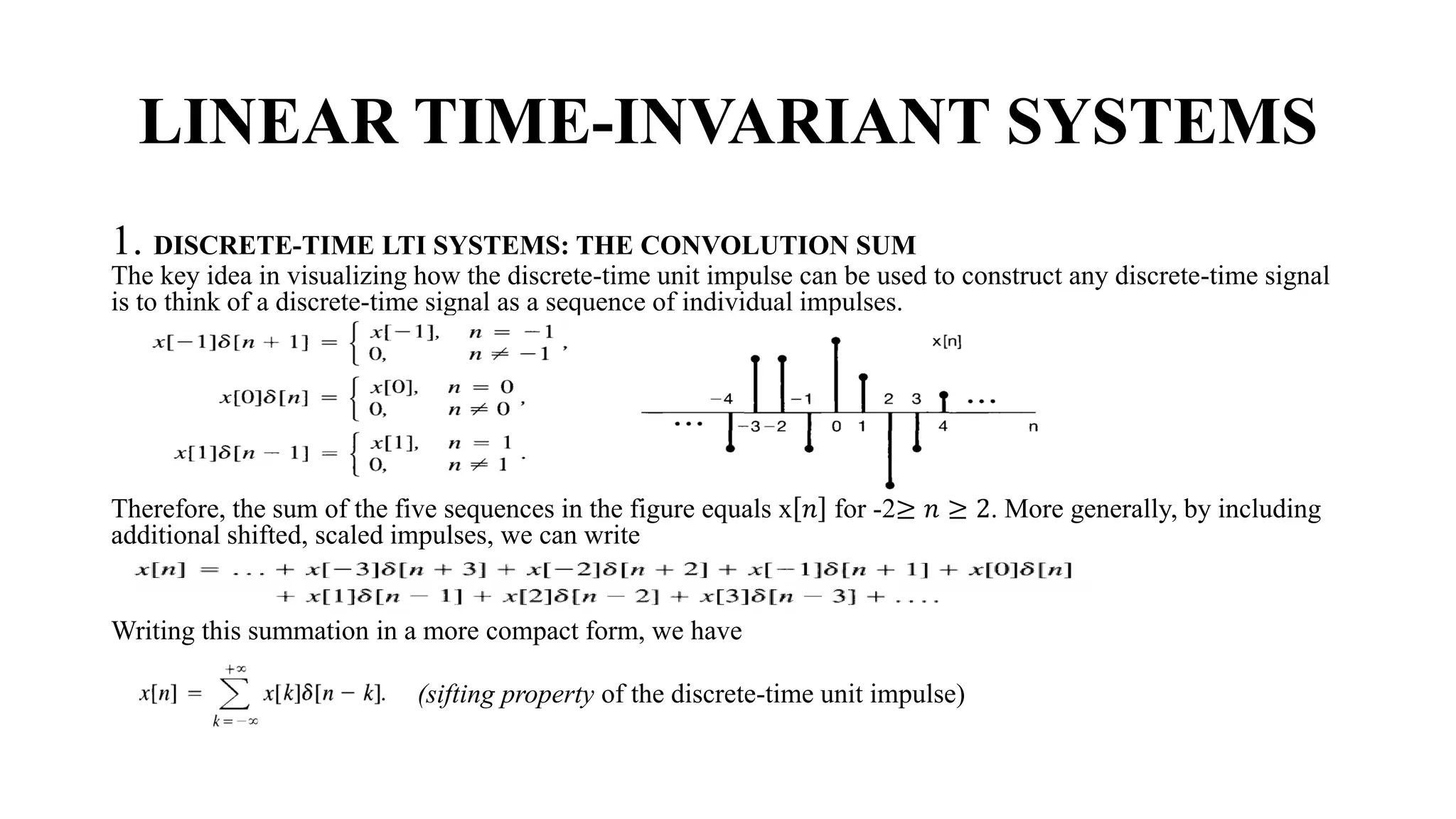
12. DISCRETE-TIME LTI SYSTEMS: THE CONVOLUTION SUM
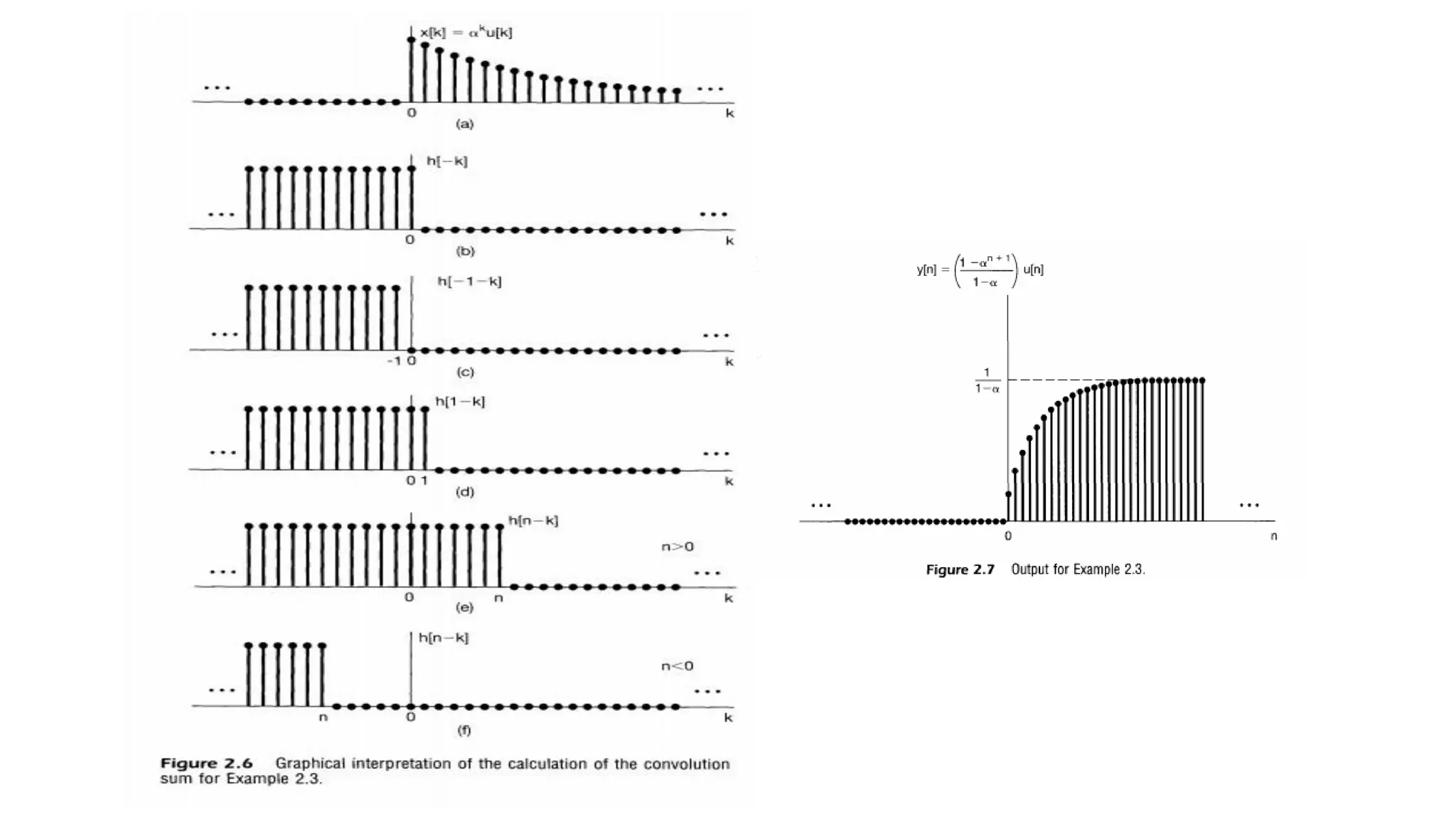
• An example, consider 𝑥 𝑛 = 𝑢 𝑛 , the unit step. In this case, since 𝑢 𝑘 = 0 for k < 0, and 𝑢 𝑘 = 1 for k ≥
0,
Because the sequence 𝛿[𝑛 − 𝑘] is nonzero only when 𝑘 = 𝑛, the summation on the righthand side of the
equation below "sifts" through the sequence of values 𝑥[𝑘] and preserves only the value corresponding to k = n.

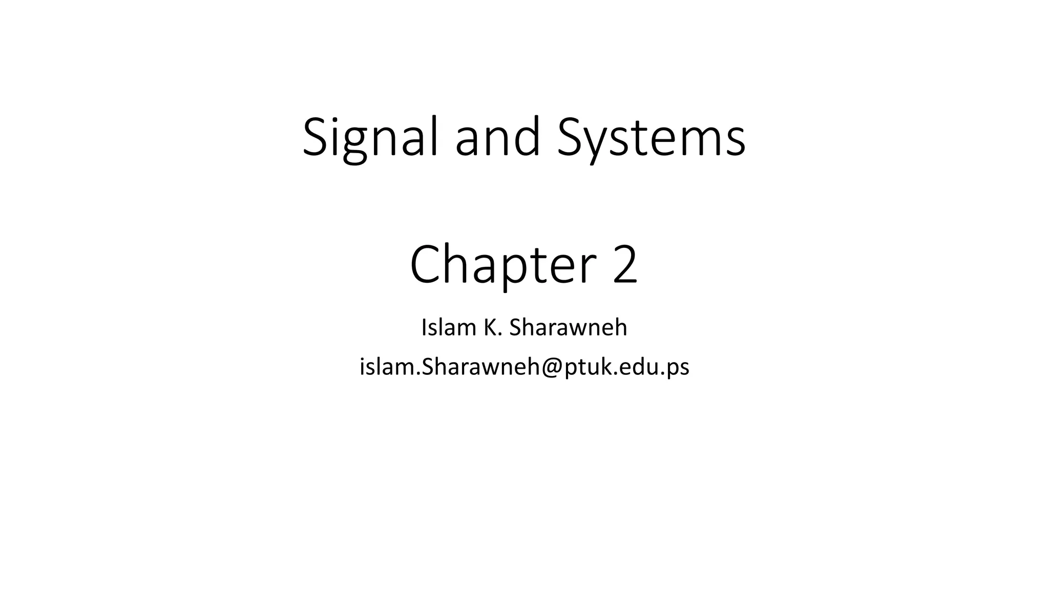
13. The Discrete-Time Unit Impulse Response and the Convolution
Sum Representation of LTI Systems
• The Discrete-Time Unit Impulse Response and the Convolution Sum Representation of LTI Systems
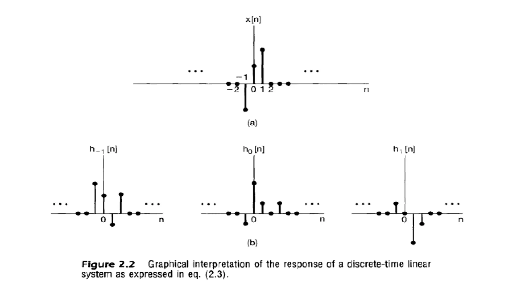
• The response of a linear system to 𝑥[𝑛] will be the superposition of the scaled responses of the system to each of
these shifted impulses.
• Moreover, the property of time invariance tells us that the responses of a time-invariant system to the time-shifted
unit impulses are simply time-shifted versions of
one another.
• The convolution-sum representation for discrete-time systems that are both linear and time invariant results from
putting these two basic facts together.
• Consider the response of a linear (but possibly time-varying) system to an arbitrary input 𝑥[𝑛]
• If we know the response of a linear system to the set of shifted unit impulses, we can construct the response to an
arbitrary input.

15. DISCRETE-TIME LTI SYSTEMS: THE CONVOLUTION SUM
• In general, of course, the responses ℎ𝑘[𝑛] need not be related to each other for different values of k. However,
if the linear system is also time invariant, then these responses to time-shifted unit impulses are all time-
shifted versions of each other. Specifically, since 𝛿[𝑛 − 𝑘]is a time-shifted version of 𝛿[𝑛], the response
ℎ𝑘[𝑛] is a time-shifted version of ℎ0[𝑛]; i.e.,
• For notational convenience, we will drop the subscript on ℎ0[𝑛] and define the unit impulse (sample) response
• That is, h[n] is the output of the LTI system when 𝛿[𝑛] is the input. Then for an LTI system.
This result is referred to as the convolution sum or superposition
sum. We will represent the operation of convolution
symbolically as

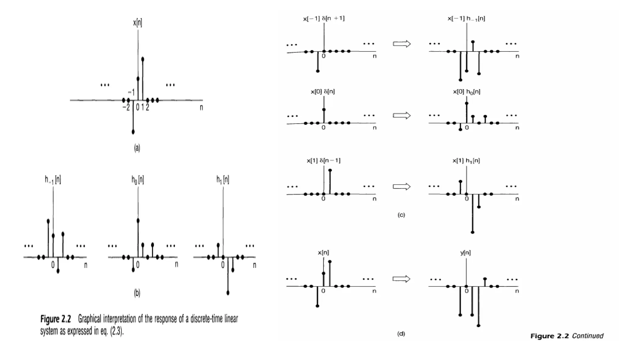
17. DISCRETE-TIME LTI SYSTEMS: THE CONVOLUTION SUM
• The convolution sum expresses the response of an LTI system to an arbitrary input in terms of the system's
response to the unit impulse. From this, we see that an LTI system is completely characterized by its response
to a single signal, namely, its response to the unit impulse.
• In the case of an LTI system, the response due to the input 𝑥 𝑘 applied at 𝑘 time is 𝑥 𝑘 ℎ 𝑛 − 𝑘 ; i.e., it is a
shifted and scaled version (an "echo") of ℎ[𝑛]. As before, the actual output is the superposition of all these
responses.

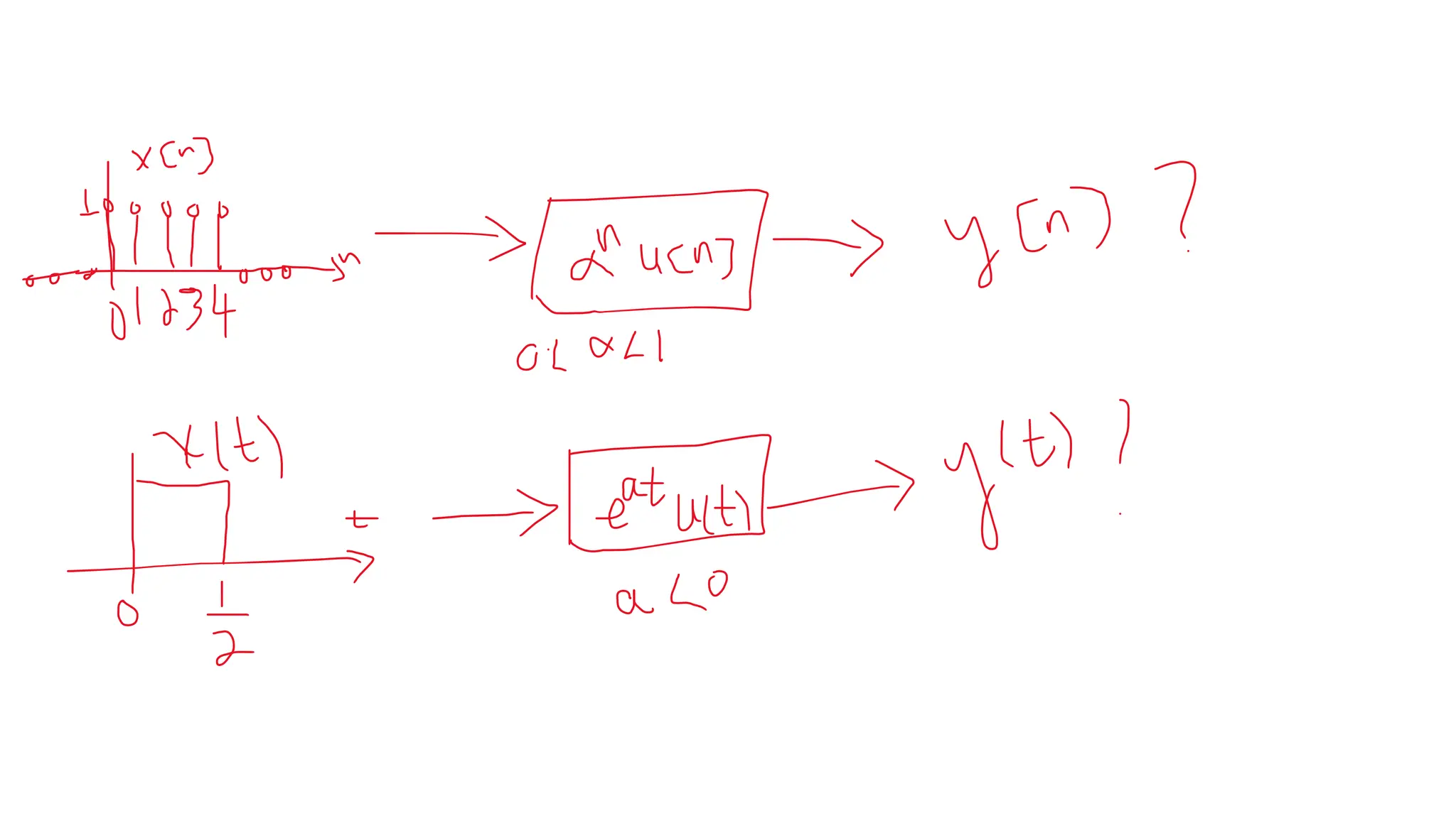
18. DISCRETE-TIME LTI SYSTEMS: THE CONVOLUTION SUM
• Consider an input x 𝑛 and a unit impulse response ℎ[𝑛] given by

22. CONTINUOUS-TIME LTI SYSTEMS: THE CONVOLUTION INTEGRAL
2. CONTINUOUS-TIME LTI SYSTEMS: THE
CONVOLUTION INTEGRAL
For a CT system
𝑥 𝑡 = න
−∞
∞
𝑥(𝜏)𝛿 𝑡 − 𝜏 𝑑𝜏
If the system is linear
𝑦 𝑡 = න
−∞
∞
𝑥 𝜏 ℎ𝜏 𝑡 𝑑𝜏
In case of time invariant system
ℎ𝜏 𝑡 = ℎ 𝑡 − 𝜏
𝑦 𝑡 = න
−∞
∞
𝑥 𝜏 ℎ 𝑡 − 𝜏 𝑑𝜏
This result is referred to as the convolution integral or
superposition integral. We will represent the operation
of convolution symbolically as
𝑥(𝑡) 𝑦(𝑡)
CT system
𝑥 𝑡 = 𝛿(𝑡 − 𝜏) 𝑦 𝑡 = ℎ𝜏(𝑡)
CT system