Downloaded 61 times
![39 LabVIEW MathScript
Tutorial: Control and Simulation in LabVIEW
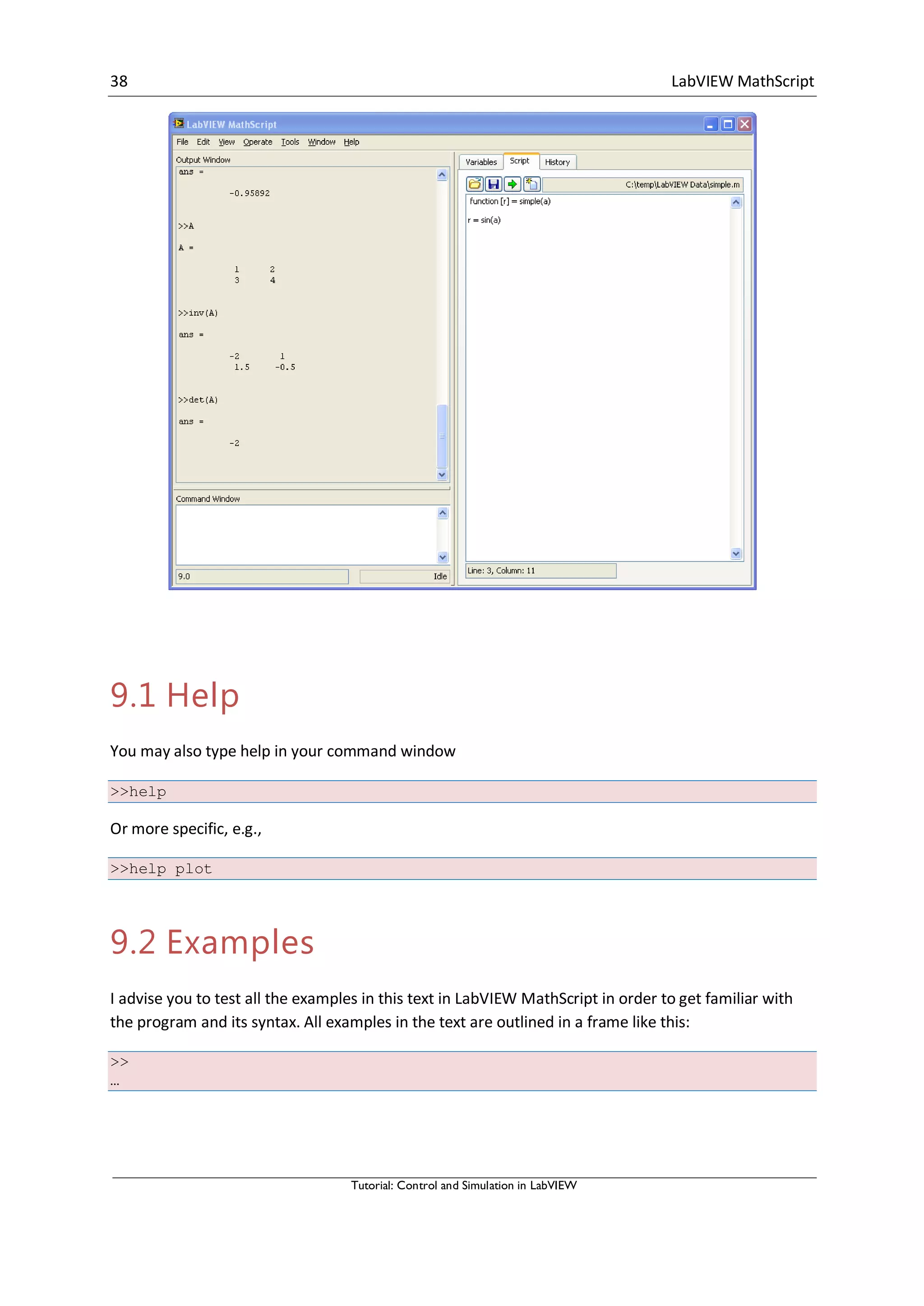
This is commands you should write in the Command Window.
You type all your commands in the Command Window. I will use the symbol “>>” to illustrate that
the commands should be written in the Command Window.
Example: Matrices
Defining the following matrix
[ ]
The syntax is as follows:
>> A = [1 2;0 3]
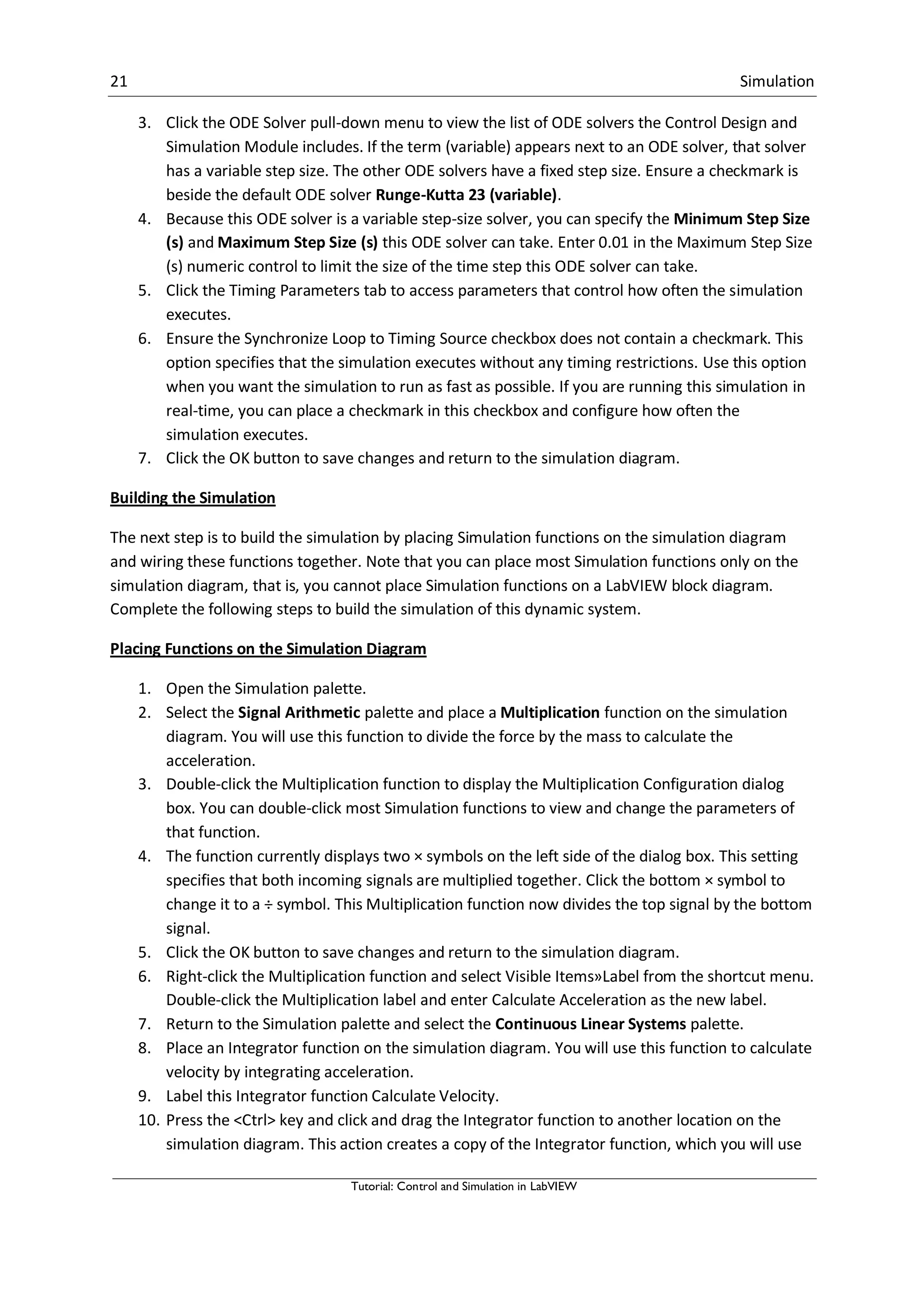
Or
>> A = [1,2;0,3]
If you, for an example, want to find the answer to
>>a=4
>>b=3
>>a+b
MathScript then responds:
ans =
7
MathScript provides a simple way to define simple arrays using the syntax:
“init:increment:terminator”. For instance:
>> array = 1:2:9
array =
1 3 5 7 9
defines a variable named array (or assigns a new value to an existing variable with the name array)
which is an array consisting of the values 1, 3, 5, 7, and 9. That is, the array starts at 1 (the init value),
increments with each step from the previous value by 2 (the increment value), and stops once it
reaches (or to avoid exceeding) 9 (the terminator value).
The increment value can actually be left out of this syntax (along with one of the colons), to use a
default value of 1.
>> ari = 1:5
ari =
1 2 3 4 5](https://image.slidesharecdn.com/controlandsimulationinlabview-150526005923-lva1-app6892/75/Control-and-simulation-in-lab-view-43-2048.jpg)
![40 LabVIEW MathScript
Tutorial: Control and Simulation in LabVIEW
assigns to the variable named ari an array with the values 1, 2, 3, 4, and 5, since the default value of 1
is used as the incrementer.
Note that the indexing is one-based, which is the usual convention for matrices in mathematics. This
is atypical for programming languages, whose arrays more often start with zero.
Matrices can be defined by separating the elements of a row with blank space or comma and using a
semicolon to terminate each row. The list of elements should be surrounded by square brackets: [].
Parentheses: () are used to access elements and subarrays (they are also used to denote a function
argument list).
>> A = [16 3 2 13; 5 10 11 8; 9 6 7 12; 4 15 14 1]
A =
16 3 2 13
5 10 11 8
9 6 7 12
4 15 14 1
>> A(2,3)
ans =
11
Sets of indices can be specified by expressions such as "2:4", which evaluates to [2, 3, 4]. For
example, a submatrix taken from rows 2 through 4 and columns 3 through 4 can be written as:
>> A(2:4,3:4)
ans =
11 8
7 12
14 1
A square identity matrix of size n can be generated using the function eye, and matrices of any size
with zeros or ones can be generated with the functions zeros and ones, respectively.
>> eye(3)
ans =
1 0 0
0 1 0
0 0 1
>> zeros(2,3)
ans =
0 0 0
0 0 0
>> ones(2,3)
ans =
1 1 1
1 1 1
9.3 Useful commands](https://image.slidesharecdn.com/controlandsimulationinlabview-150526005923-lva1-app6892/75/Control-and-simulation-in-lab-view-44-2048.jpg)
![41 LabVIEW MathScript
Tutorial: Control and Simulation in LabVIEW
Here are some useful commands:
Command Description
eye(x), eye(x,y) Identity matrix of order x
ones(x), ones(x,y) A matrix with only ones
zeros(x), zeros(x,y) A matrix with only zeros
diag([x y z]) Diagonal matrix
size(A) Dimension of matrix A
A’ Inverse of matrix A
9.4 Plotting
This chapter explains the basic concepts of creating plots in MathScript.
Topics:
Basic Plot commands
Example: Plotting
Function plot can be used to produce a graph from two vectors x and y. The code:
x = 0:pi/100:2*pi;
y = sin(x);
plot(x,y)](https://image.slidesharecdn.com/controlandsimulationinlabview-150526005923-lva1-app6892/75/Control-and-simulation-in-lab-view-45-2048.jpg)
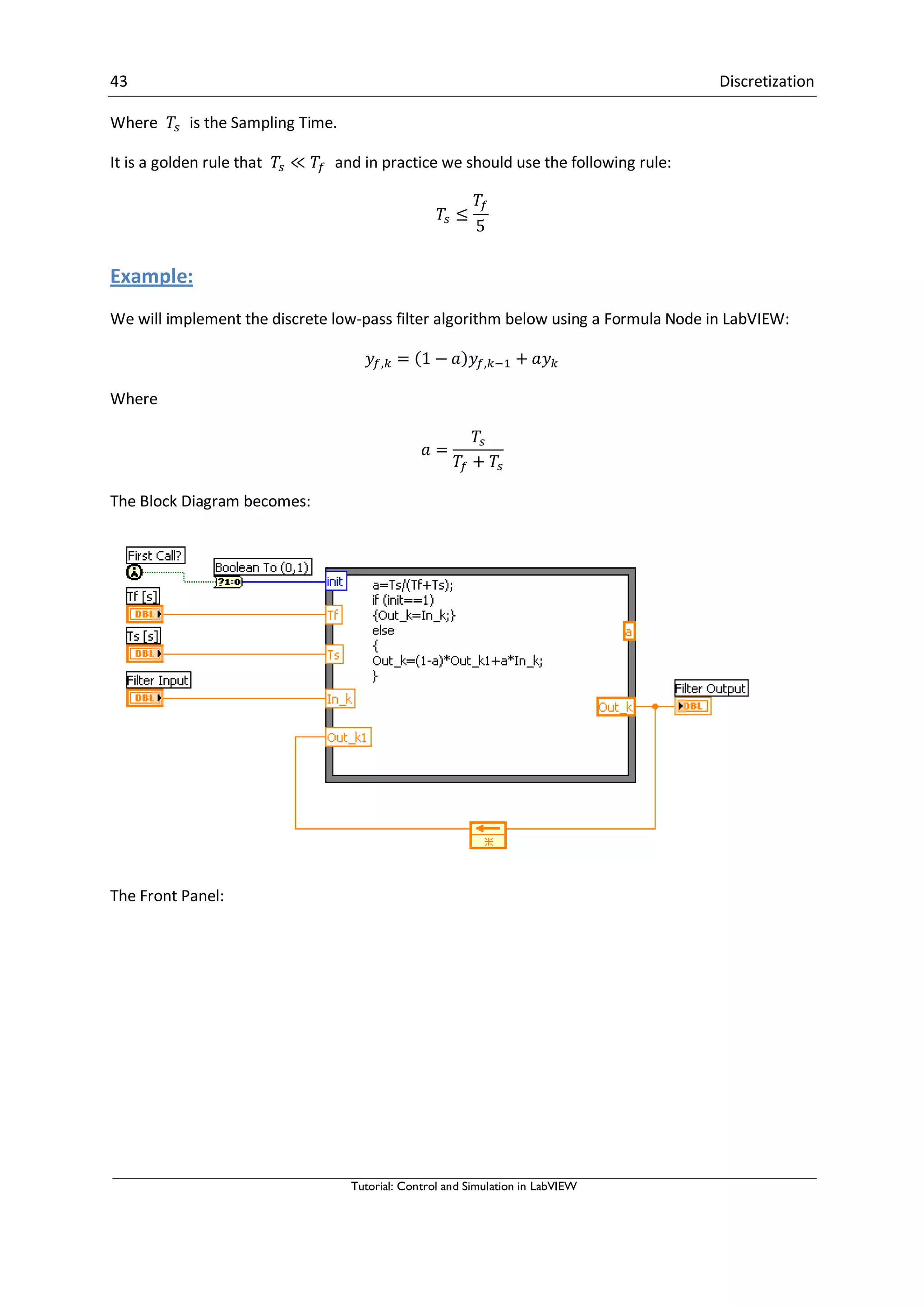
![45 Discretization
Tutorial: Control and Simulation in LabVIEW
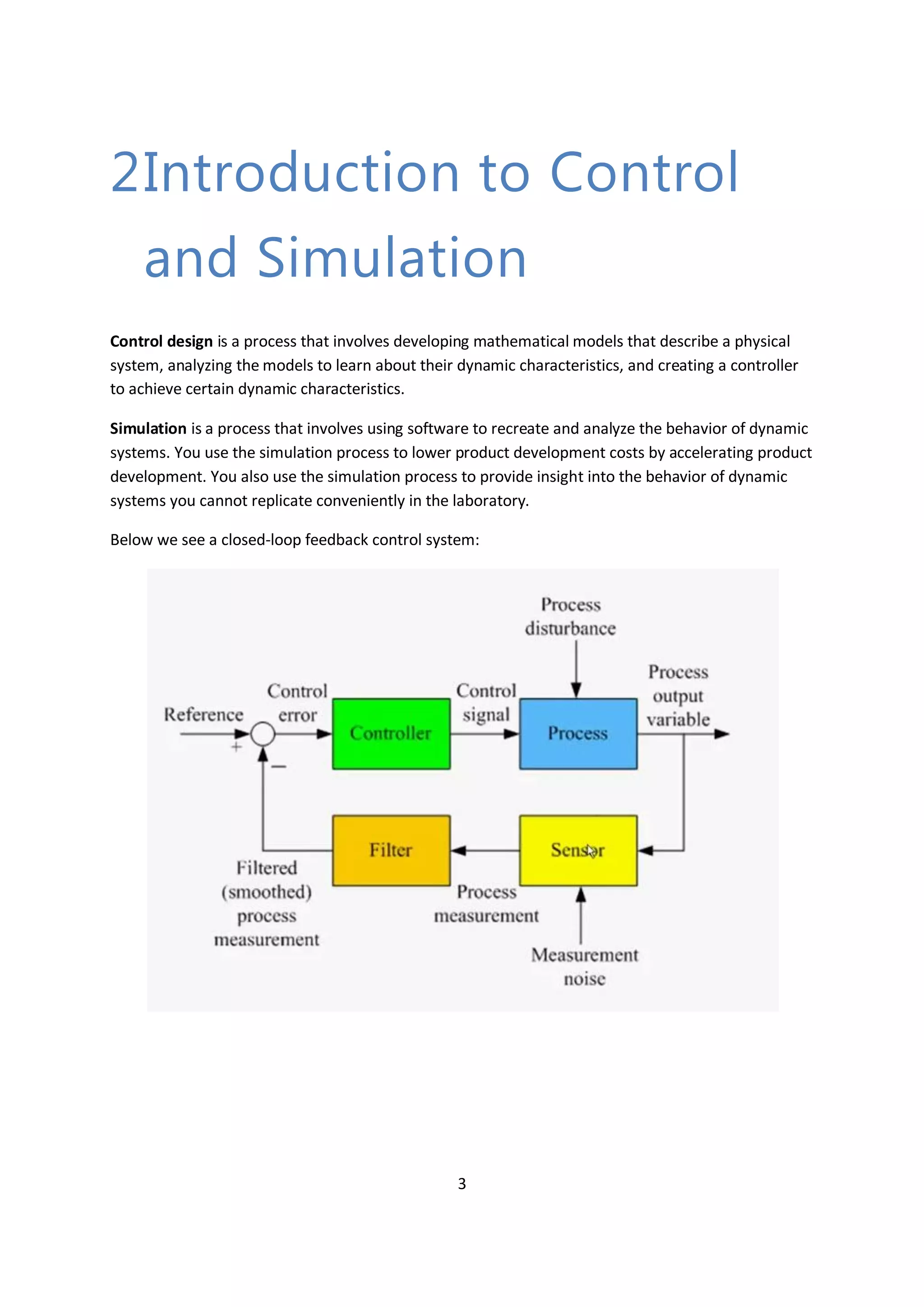
We see that the filter works fine. The red line is the unfiltered sine signal with white noise, while the
red line is the filtered results.
[End of Example]
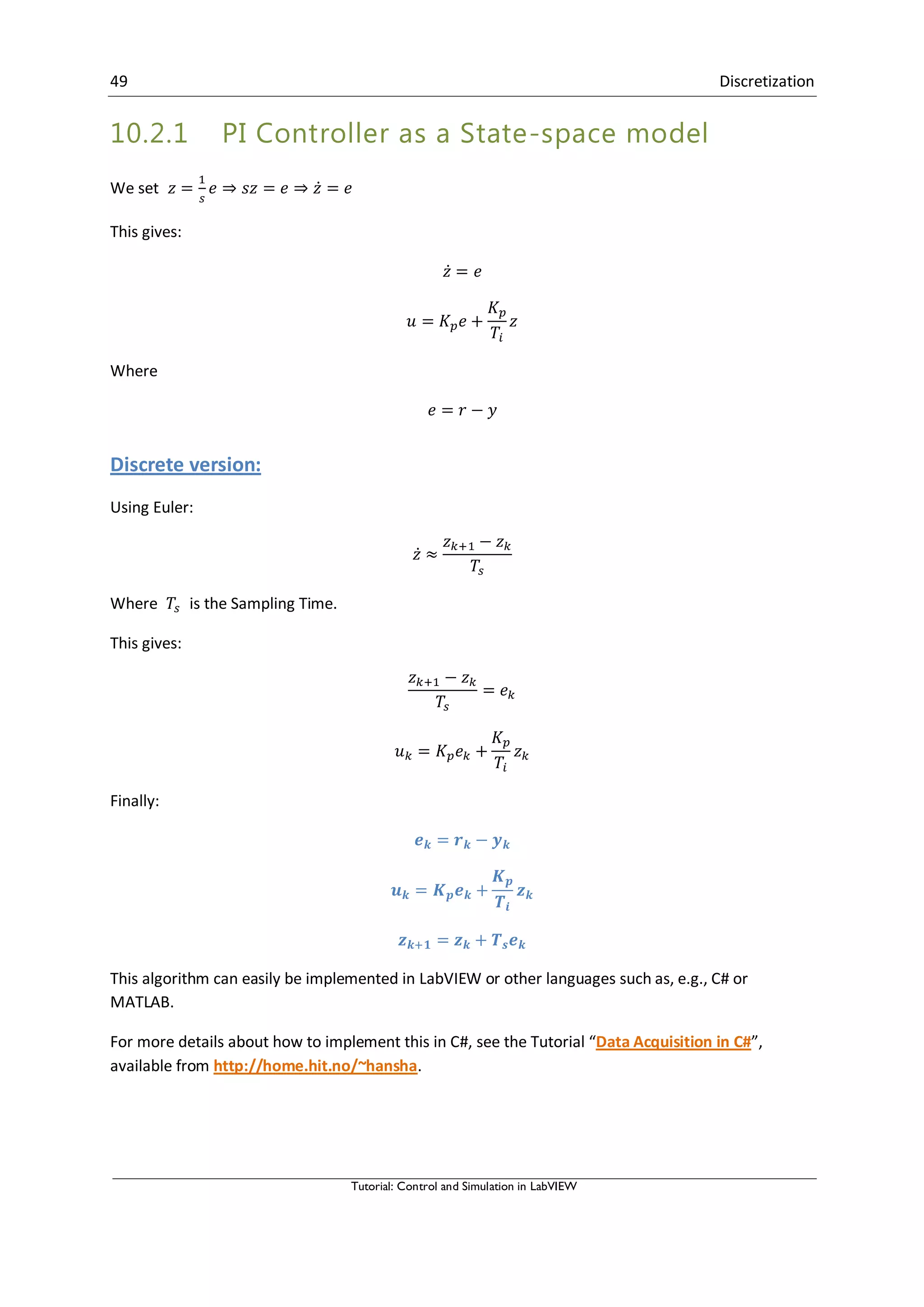
10.2 PI Controller
A PI controller may be written:
∫
Where is the controller output and is the control error:
Laplace version:
Discrete version:
We start with:](https://image.slidesharecdn.com/controlandsimulationinlabview-150526005923-lva1-app6892/75/Control-and-simulation-in-lab-view-49-2048.jpg)
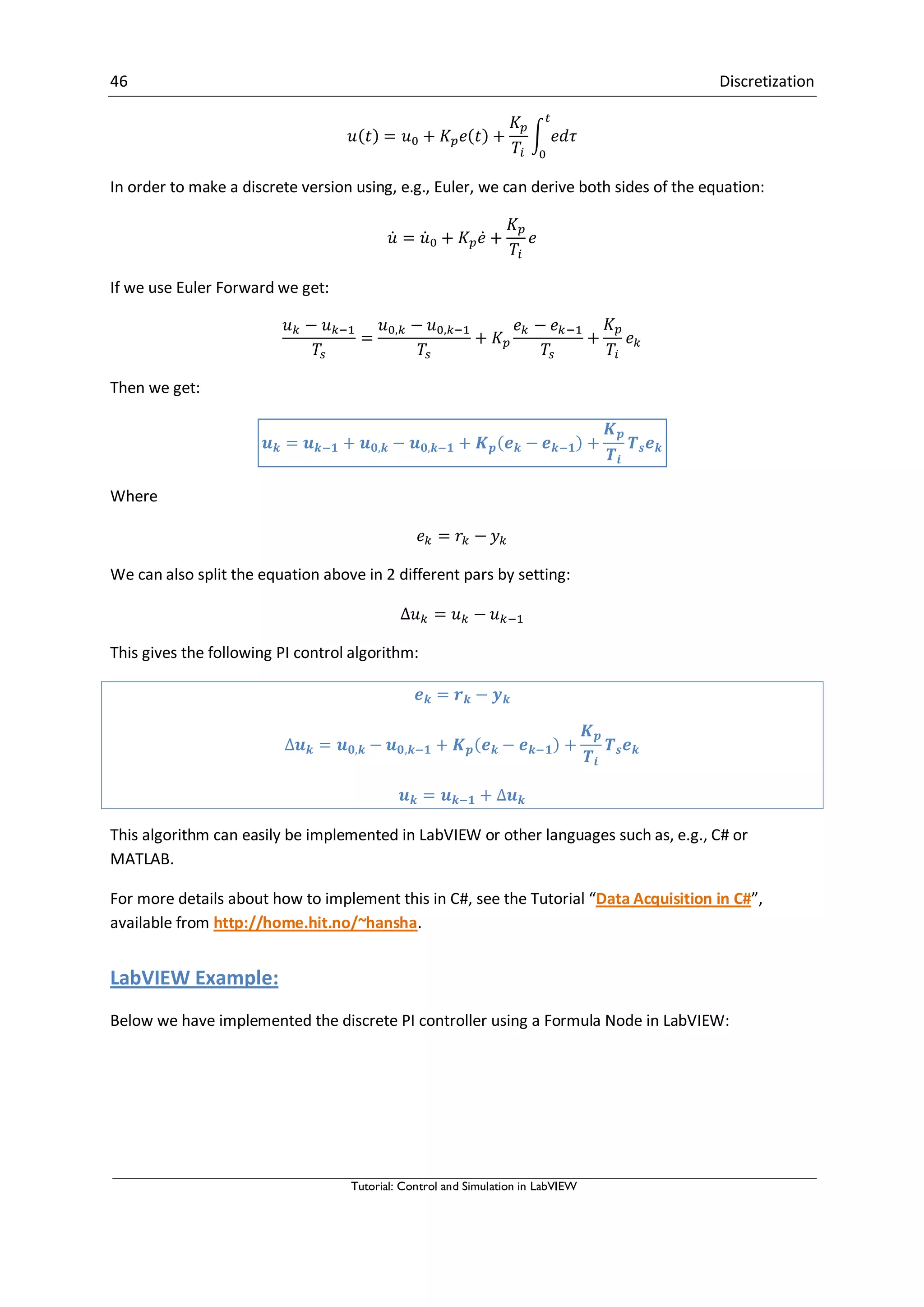
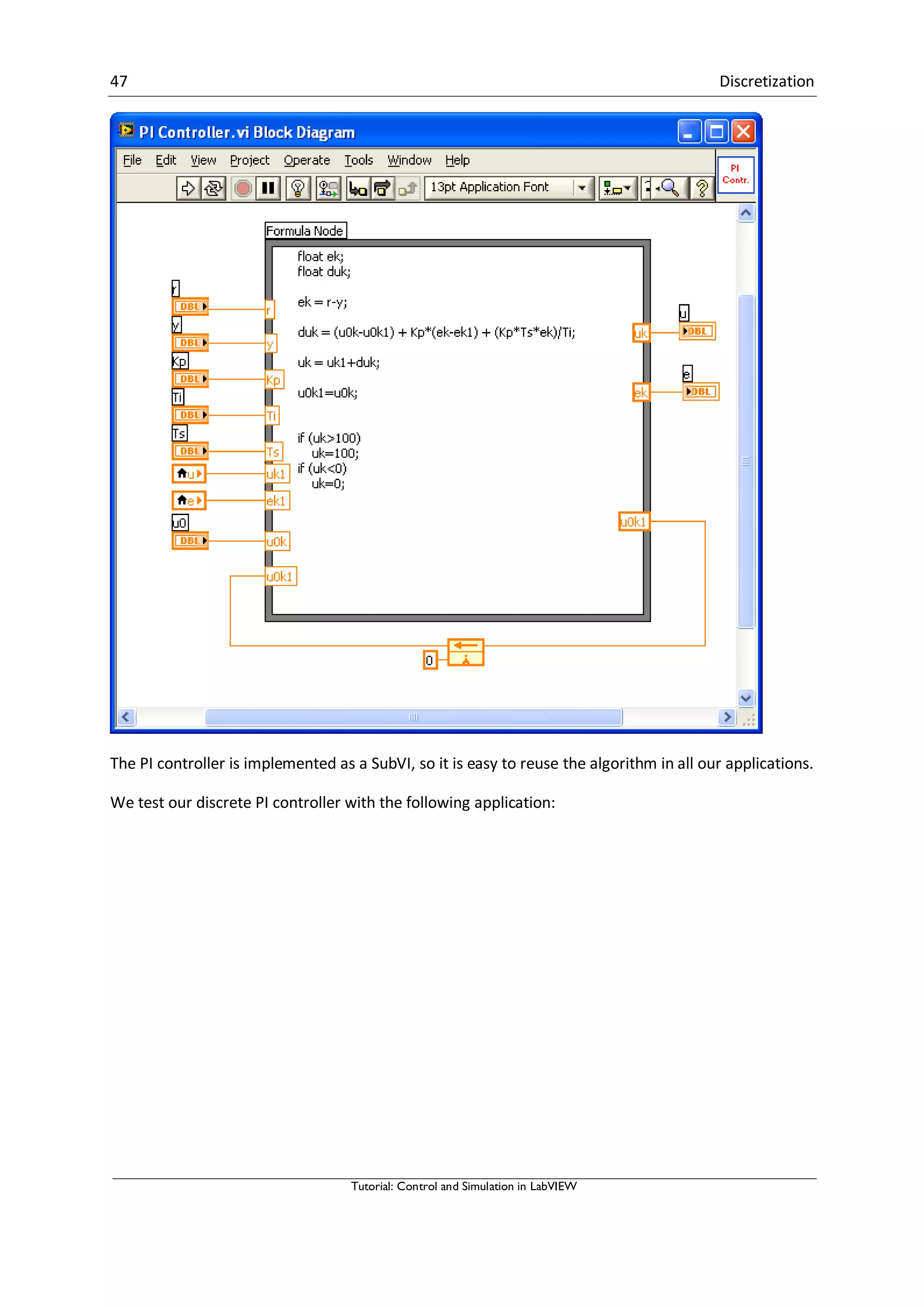
![48 Discretization
Tutorial: Control and Simulation in LabVIEW
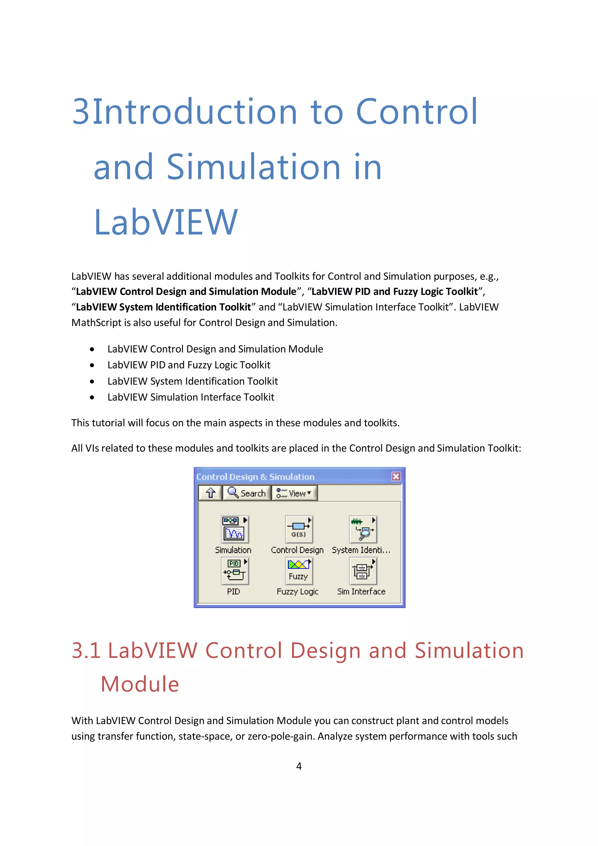
Block Diagram:
[End of Example]](https://image.slidesharecdn.com/controlandsimulationinlabview-150526005923-lva1-app6892/75/Control-and-simulation-in-lab-view-52-2048.jpg)
![50 Discretization
Tutorial: Control and Simulation in LabVIEW
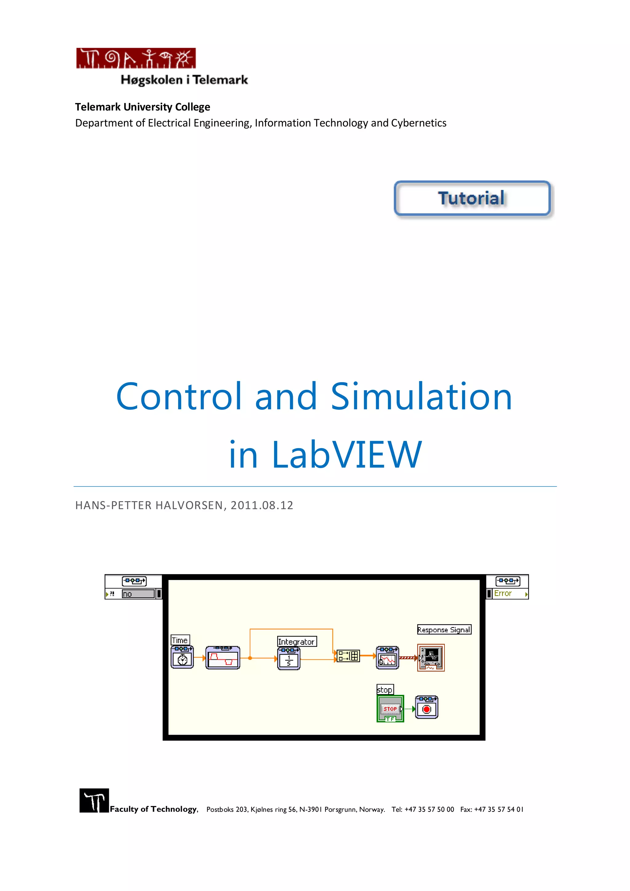
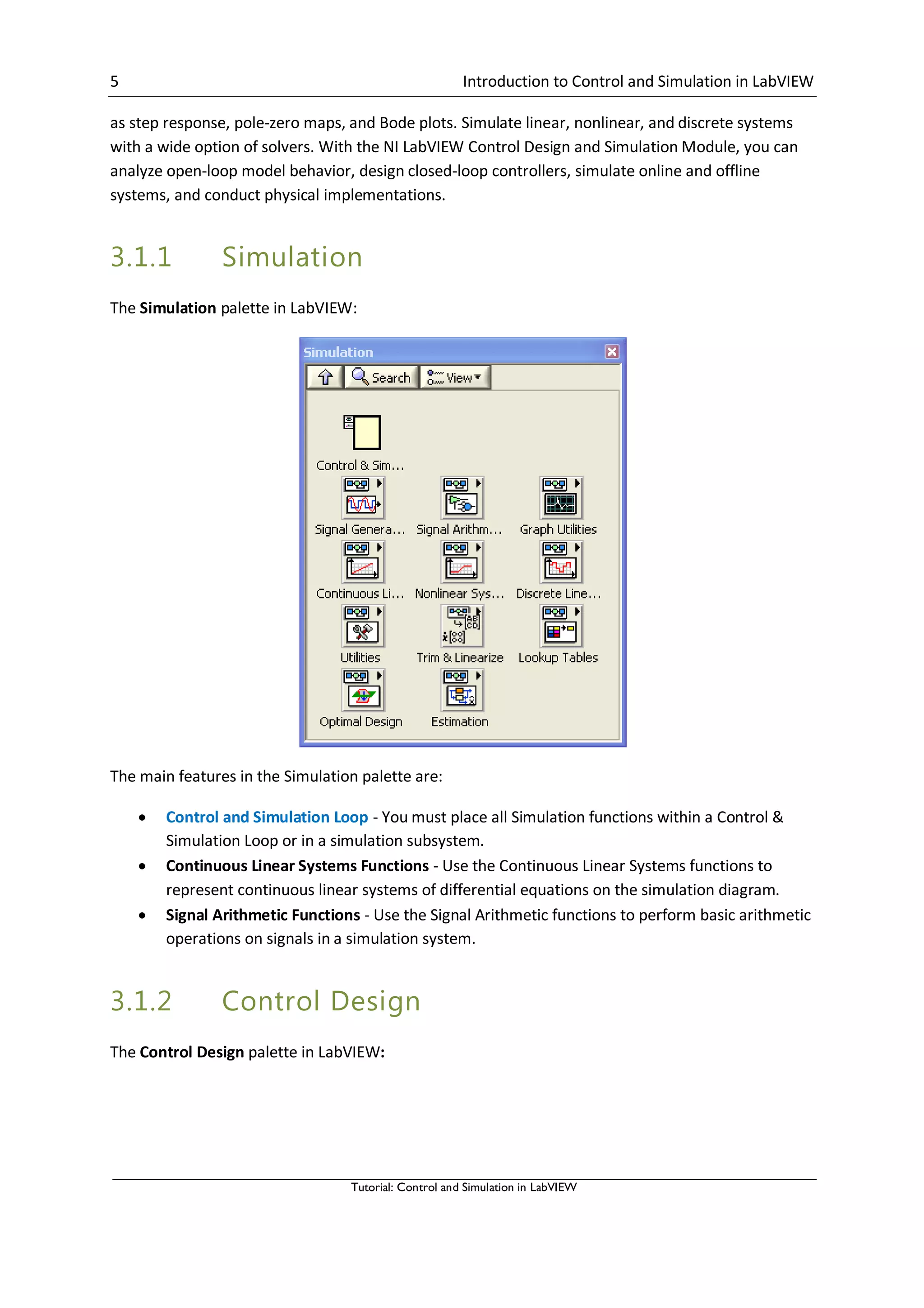
10.3 Process Model
We will use a simple water tank to illustrate how to create a discrete version of a mathematical
process model. Below we see an illustration:
A very simple (linear) model of the water tank is as follows:
̇
or
̇ [ ]
Where:
[cm] is the level in the water tank
[V] is the pump control signal to the pump
[cm2] is the cross-sectional area in the tank
[(cm3/s)/V] is the pump gain
[cm3/s] is the outflow through the valve (this outflow can be modeled more accurately
taking into account the valve characteristic expressing the relation between pressure drop
across the valve and the flow through the valve).
We can use the Euler Forward discretization method in order to create a discrete model:
̇
Then we get:](https://image.slidesharecdn.com/controlandsimulationinlabview-150526005923-lva1-app6892/75/Control-and-simulation-in-lab-view-54-2048.jpg)
![51 Discretization
Tutorial: Control and Simulation in LabVIEW
[ ]
Finally:
[ ]
This model can easily be implemented in a computer using, e.g., MATLAB, LabVIEW or C#.
For more details for how to do this in C#, see the Tutorial “Data Acquisition in C#”.
In LabVIEW this can, e.g., be implemented in a Formula Node or MathScript Node.
Example:
In this example we will simulate a Bacteria Population.
In this example we will use LabVIEW and the LabVIEW Control Design and Simulation Module to
simulate a simple model of a bacteria population in a jar.
The model is as follows:
birth rate=bx
death rate = px2
Then the total rate of change of bacteria population is:
̇
We set b=1/hour and p=0.5 bacteria-hour in our example.
We will simulate the number of bacteria in the jar after 1 hour, assuming that initially there are 100
bacteria present.
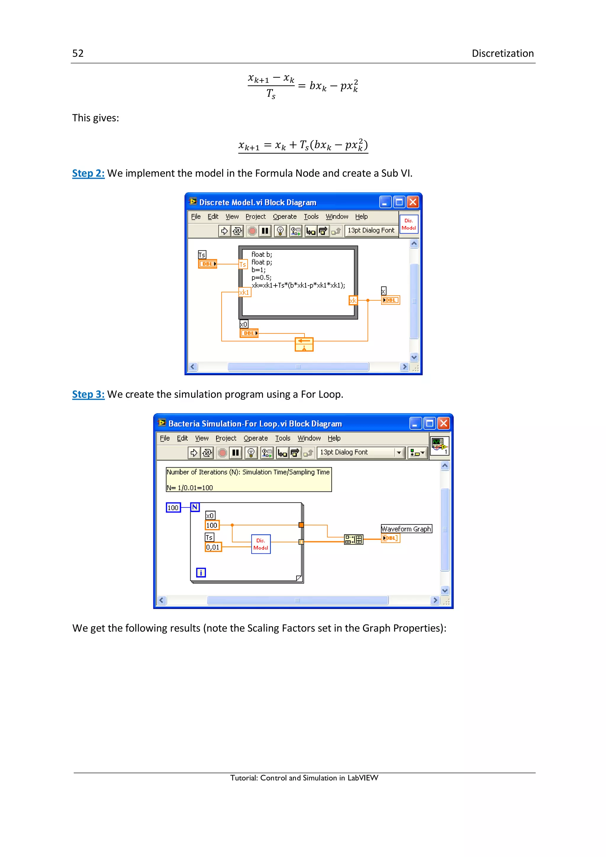
We will simulate the system using a For Loop in LabVIEW and implement the discrete model in a
Formula Node.
Step 1: We start by creating the discrete model.
If we use Euler Forward differentiation method:
̇
Where is the Sampling Time.
We get:](https://image.slidesharecdn.com/controlandsimulationinlabview-150526005923-lva1-app6892/75/Control-and-simulation-in-lab-view-55-2048.jpg)
![53 Discretization
Tutorial: Control and Simulation in LabVIEW
[End of Example]
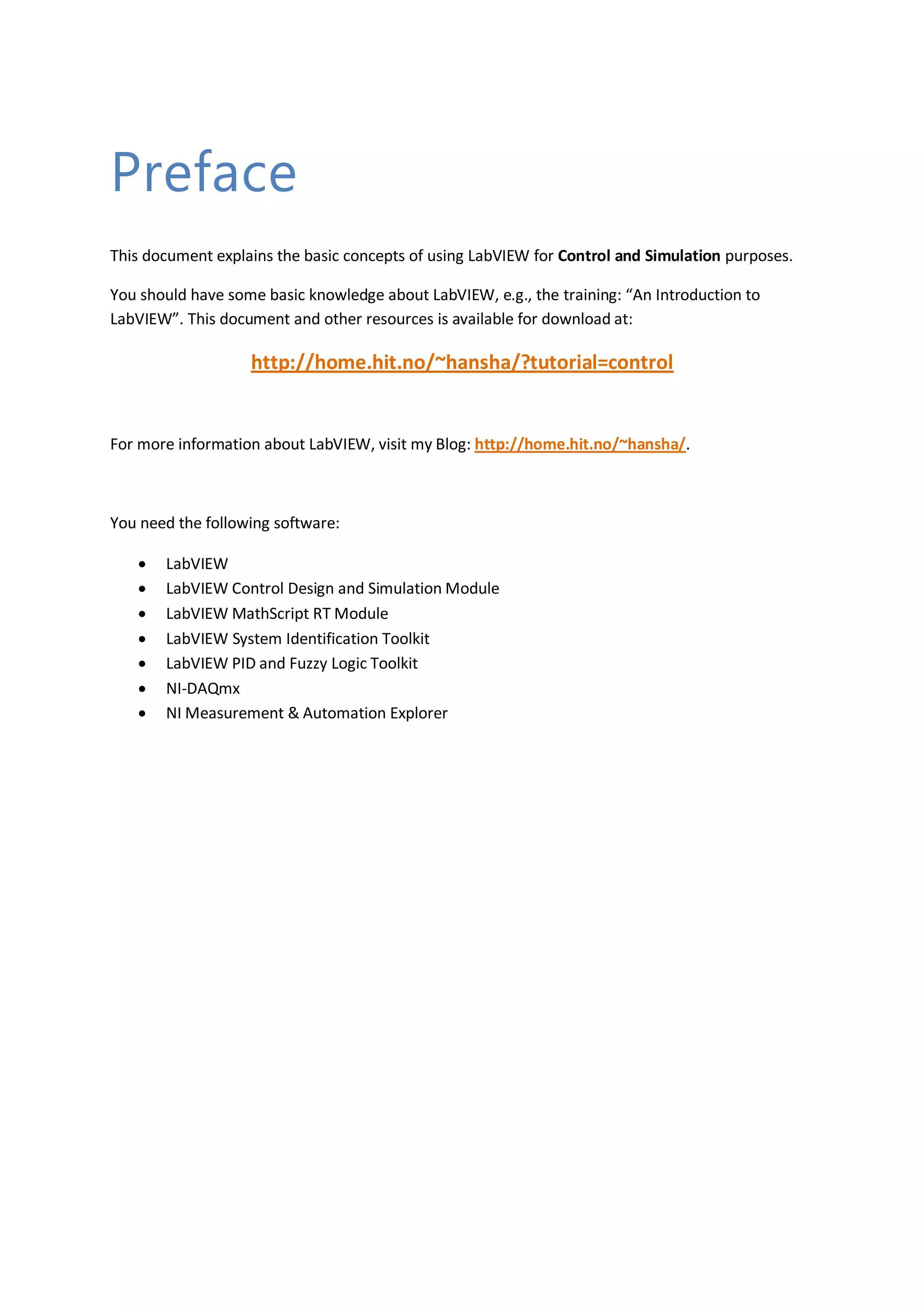
Example:
Given the following mathematical model (nonlinear):
̇ √
We will create a new application in LabVIEW where we simulate this model using a Formula Node to
implement the discrete model.
We will use the Euler Forward method (because this is a nonlinear equation):
̇
This gives:
√
[ √ ]
Block Diagram:](https://image.slidesharecdn.com/controlandsimulationinlabview-150526005923-lva1-app6892/75/Control-and-simulation-in-lab-view-57-2048.jpg)
![54 Discretization
Tutorial: Control and Simulation in LabVIEW
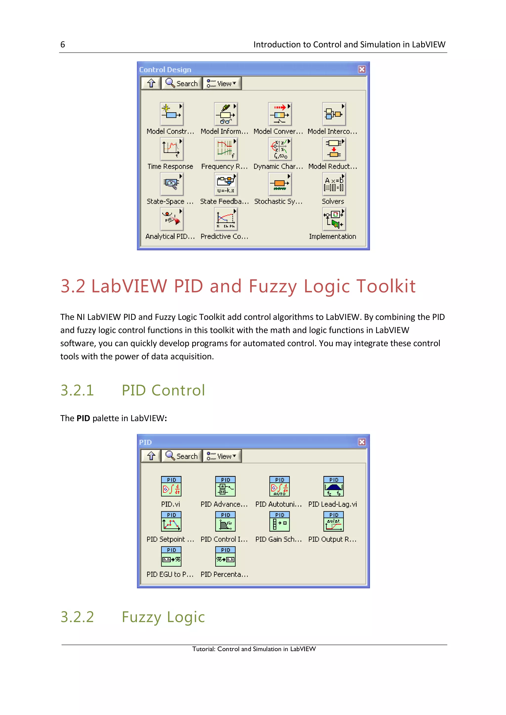
Front Panel:
[End of Example]](https://image.slidesharecdn.com/controlandsimulationinlabview-150526005923-lva1-app6892/75/Control-and-simulation-in-lab-view-58-2048.jpg)

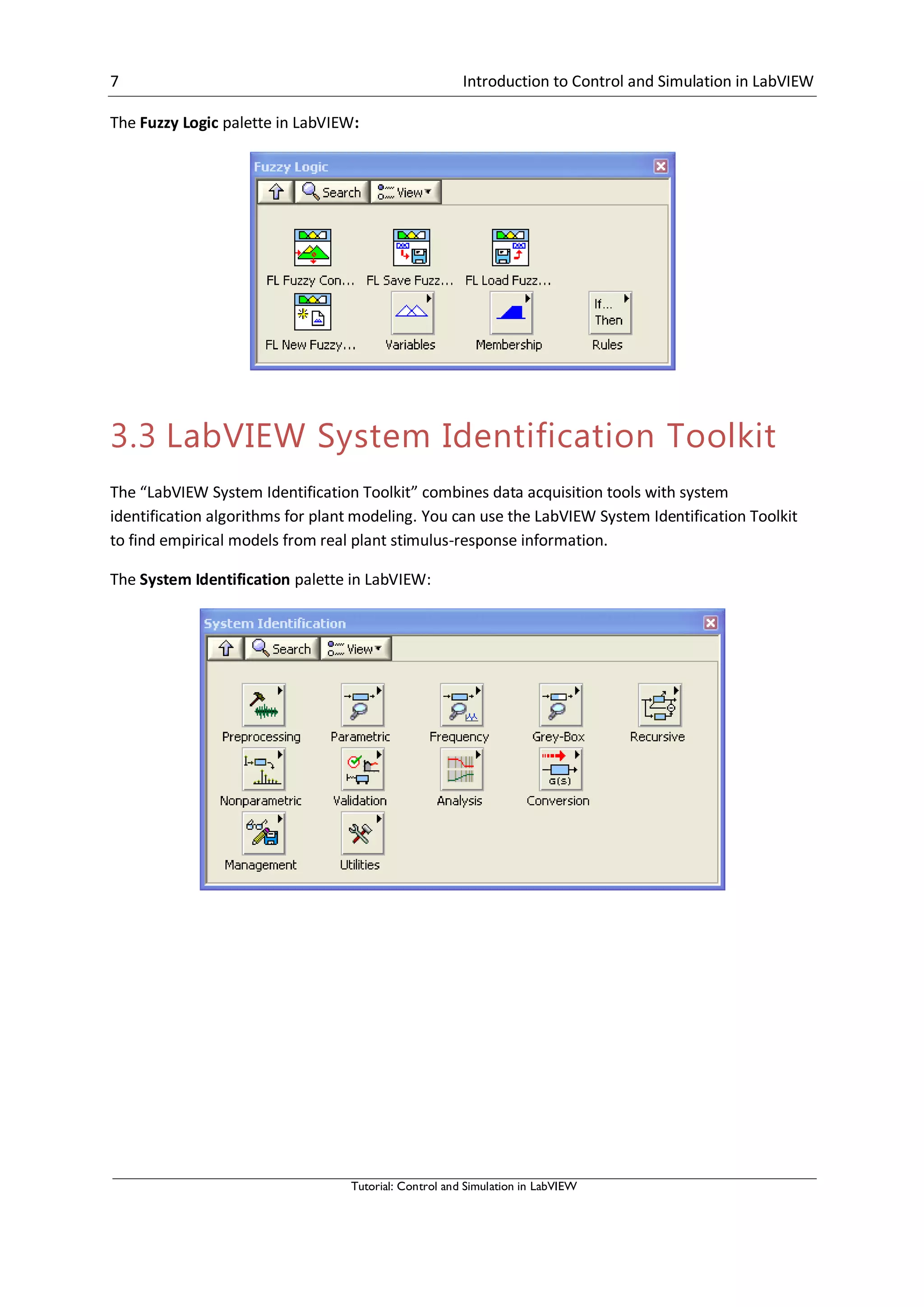
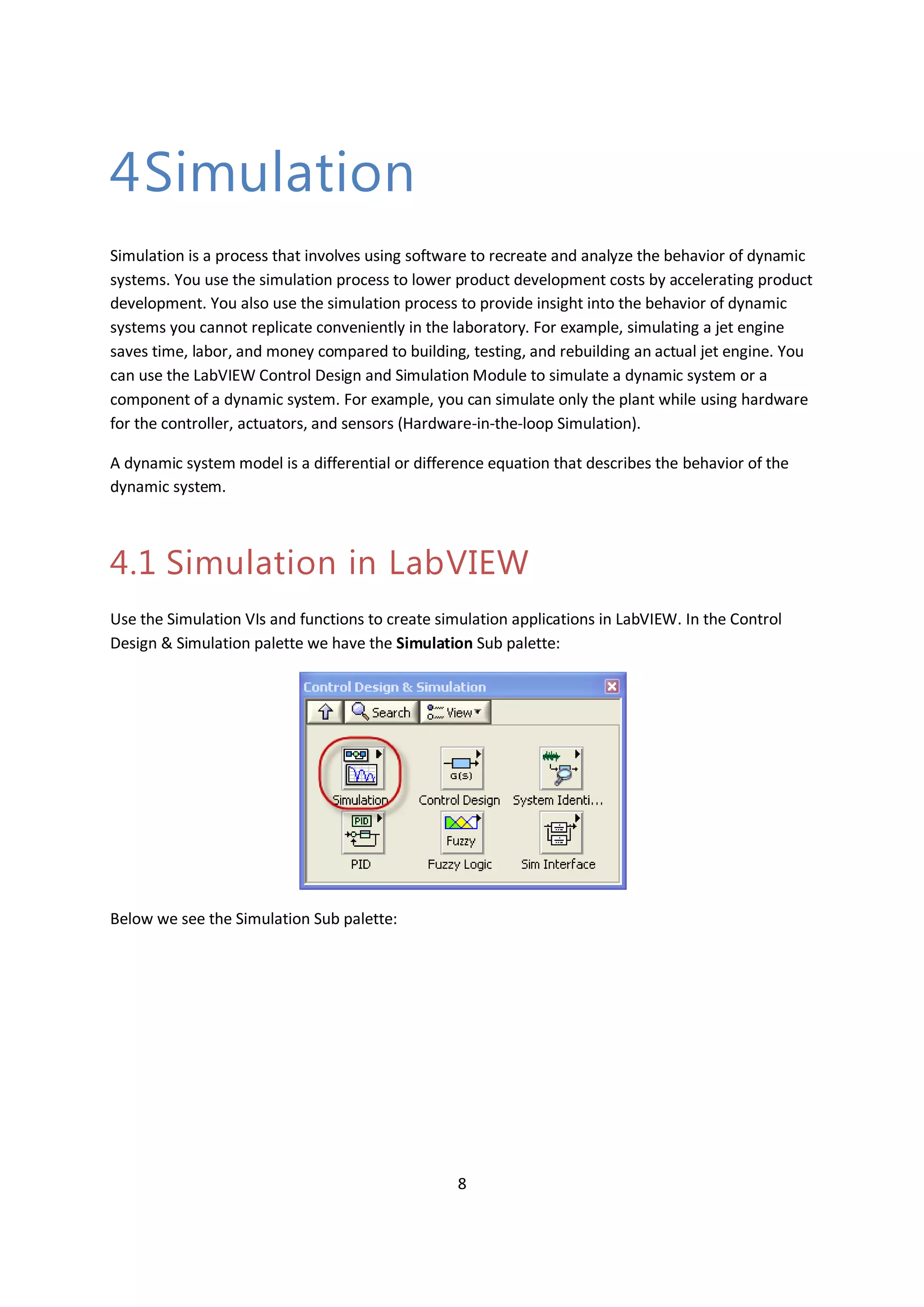
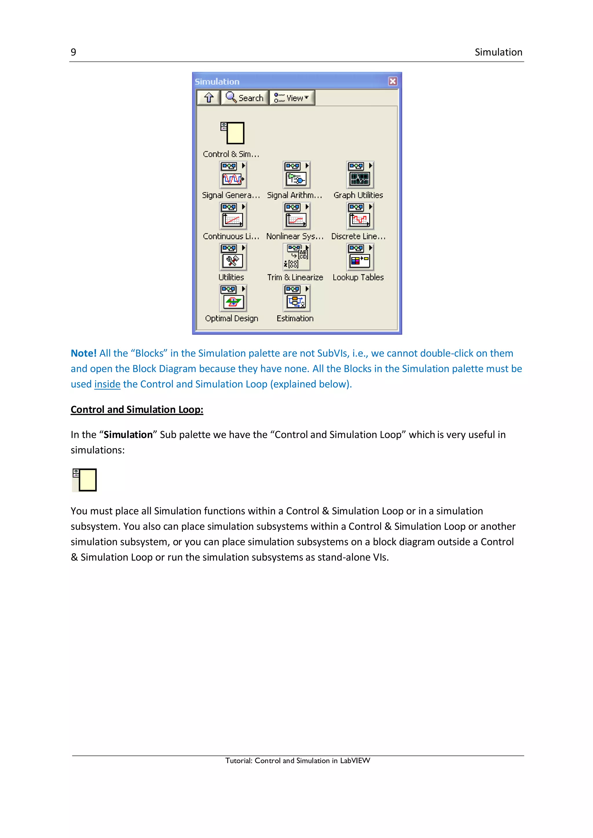
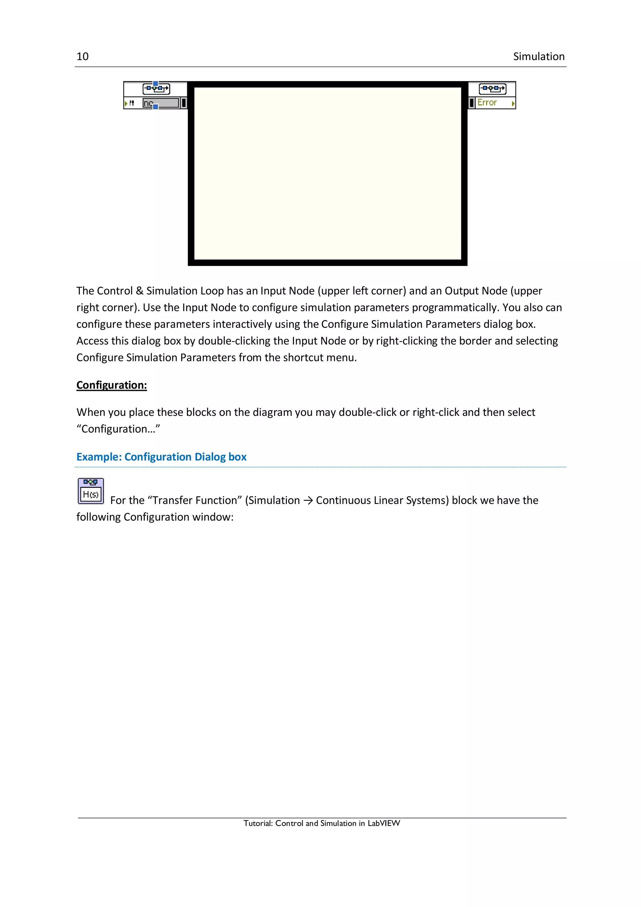
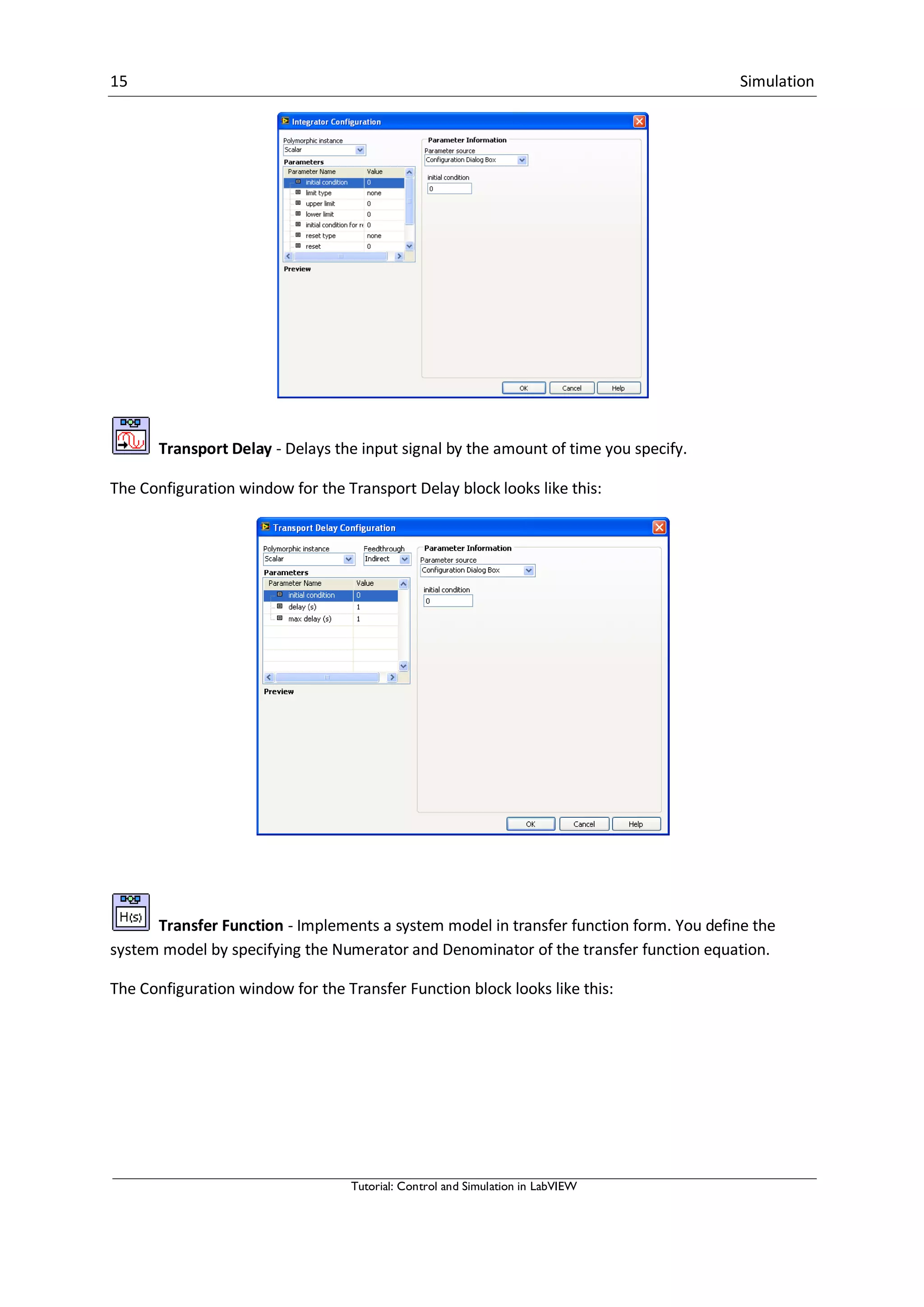
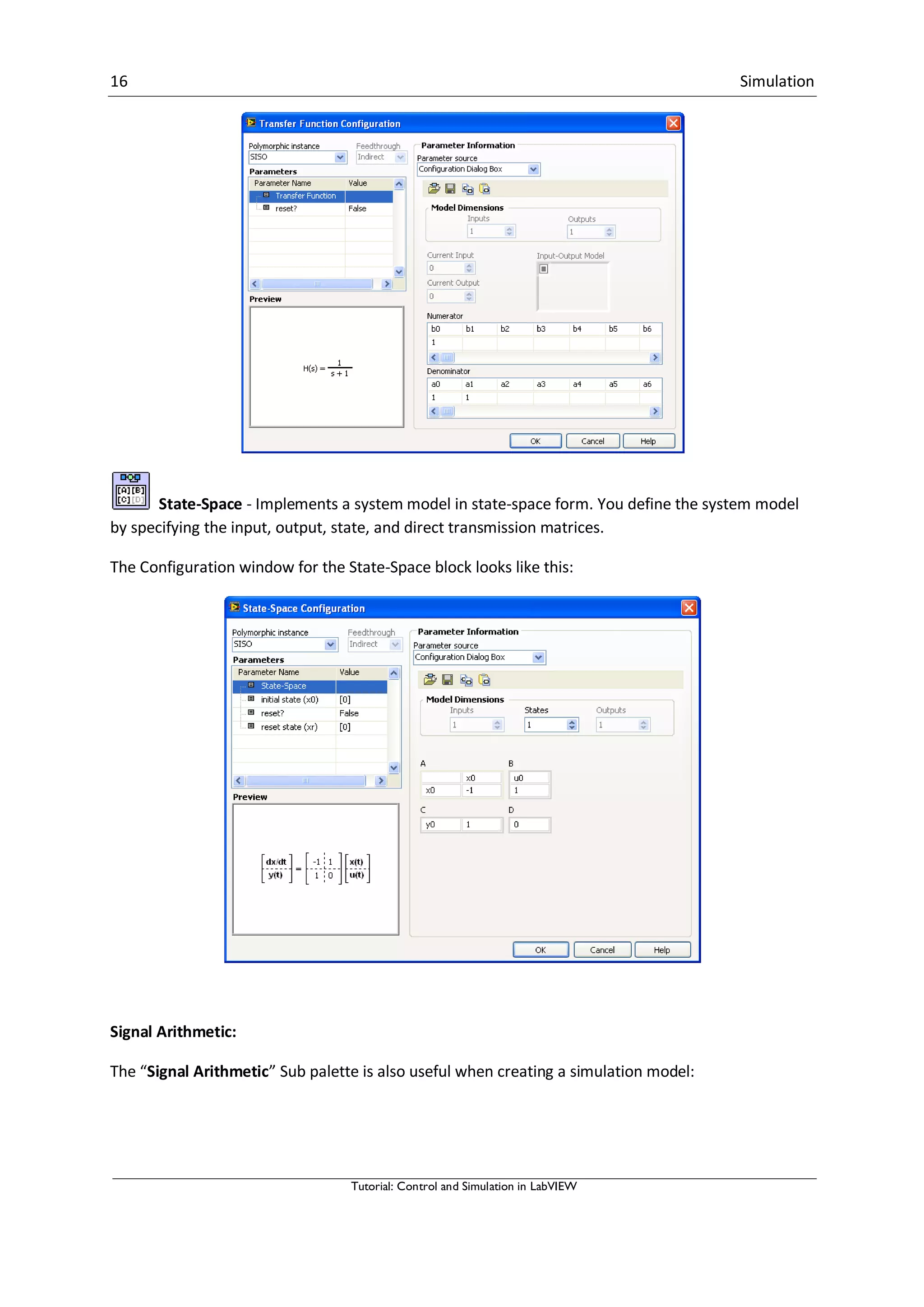
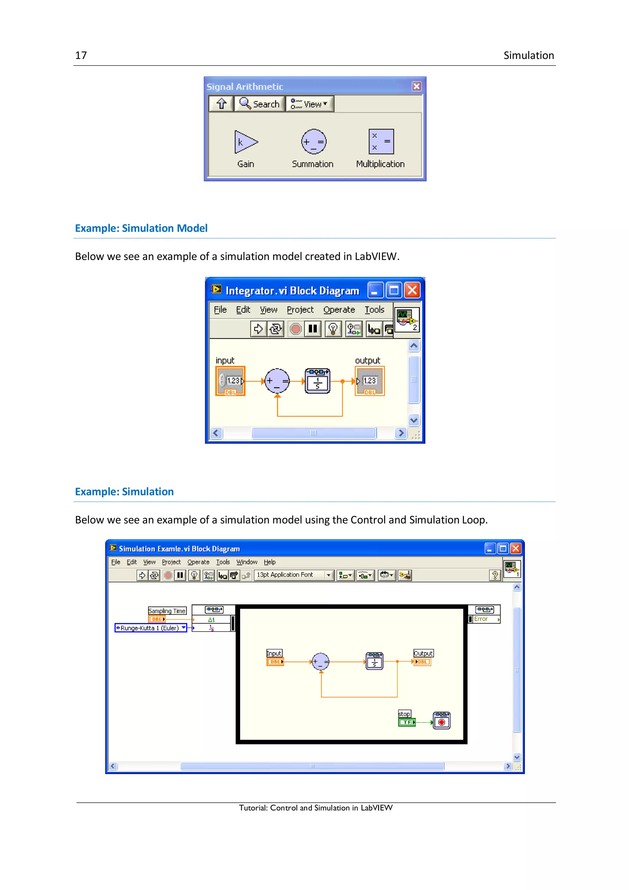
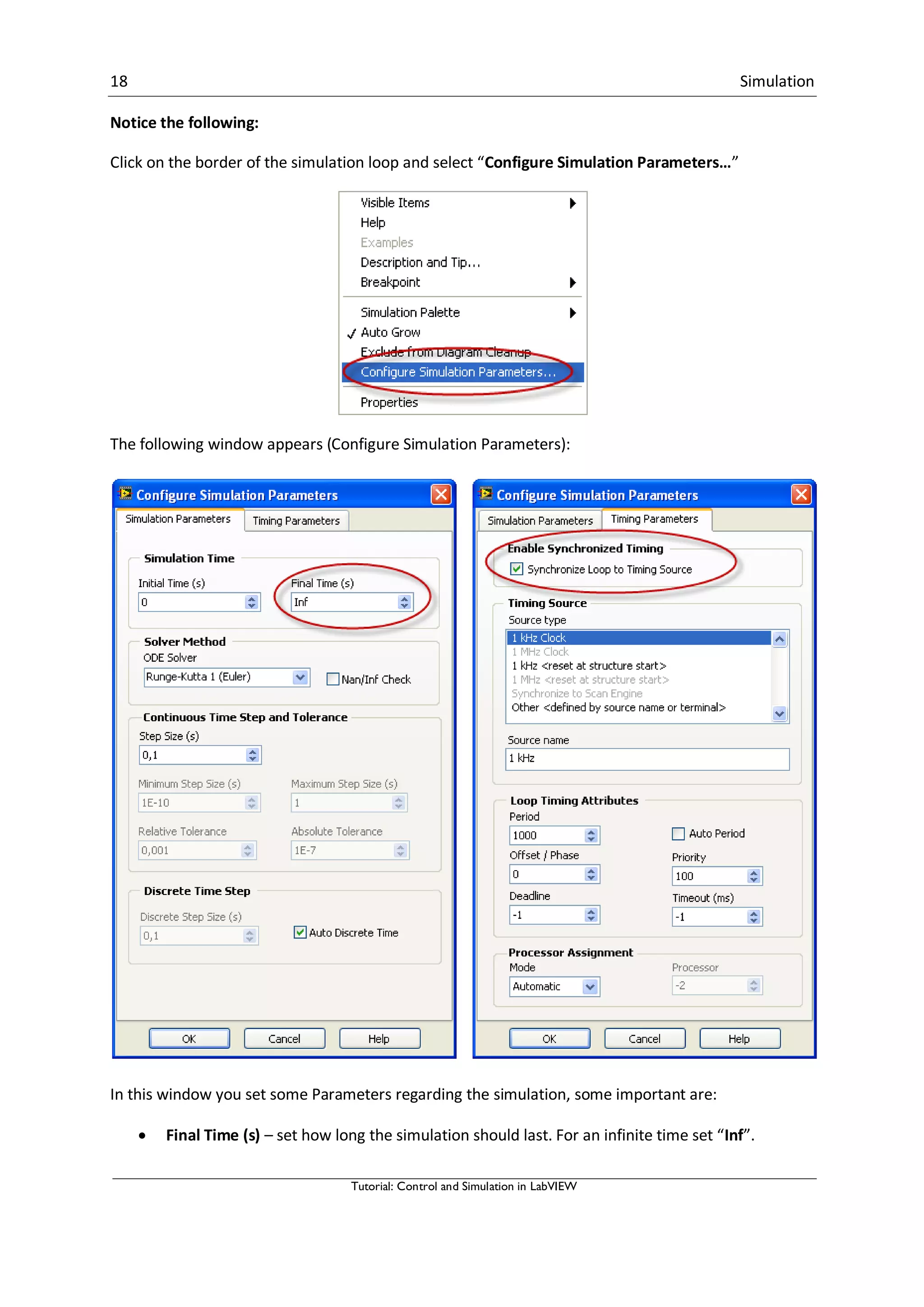
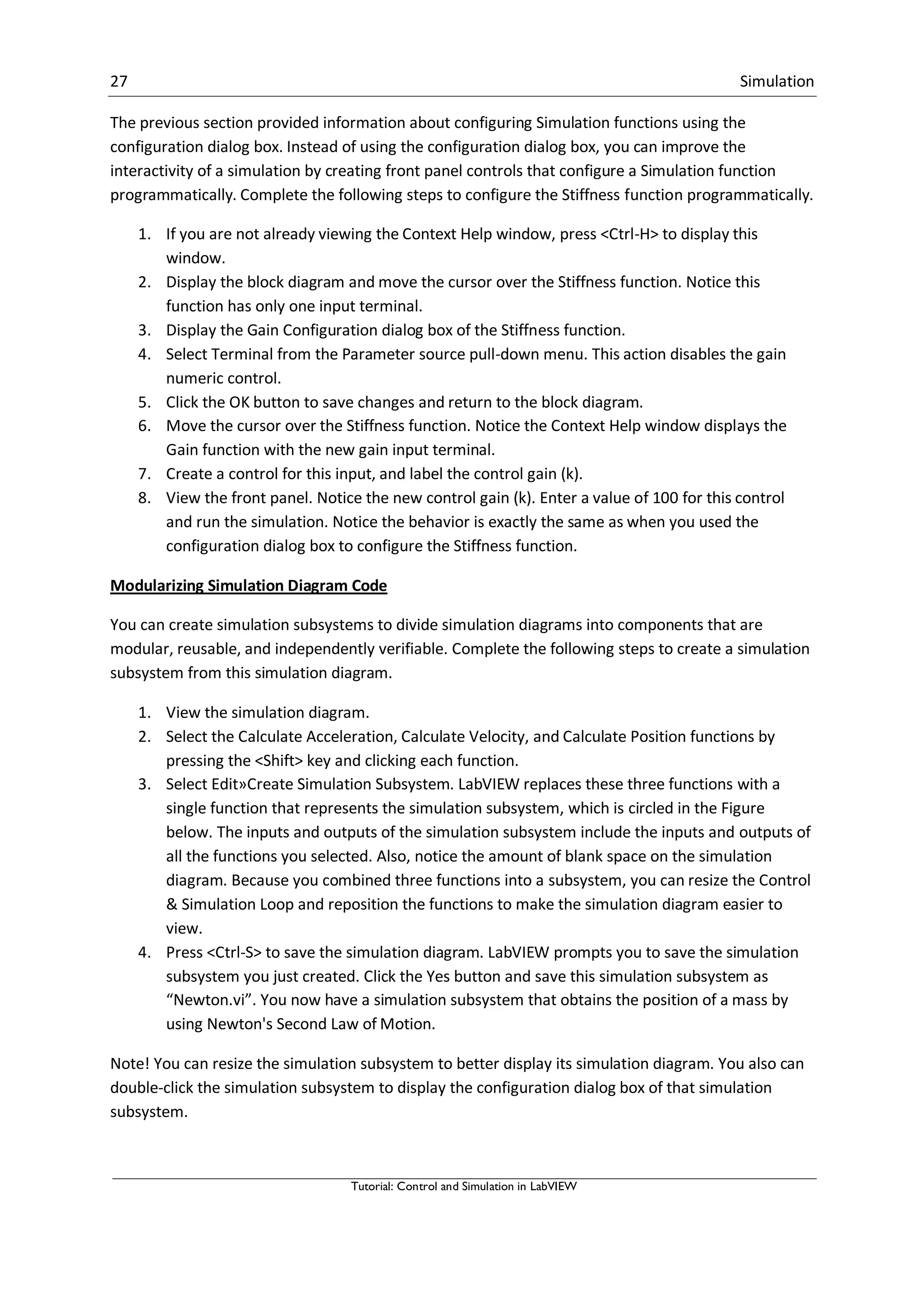
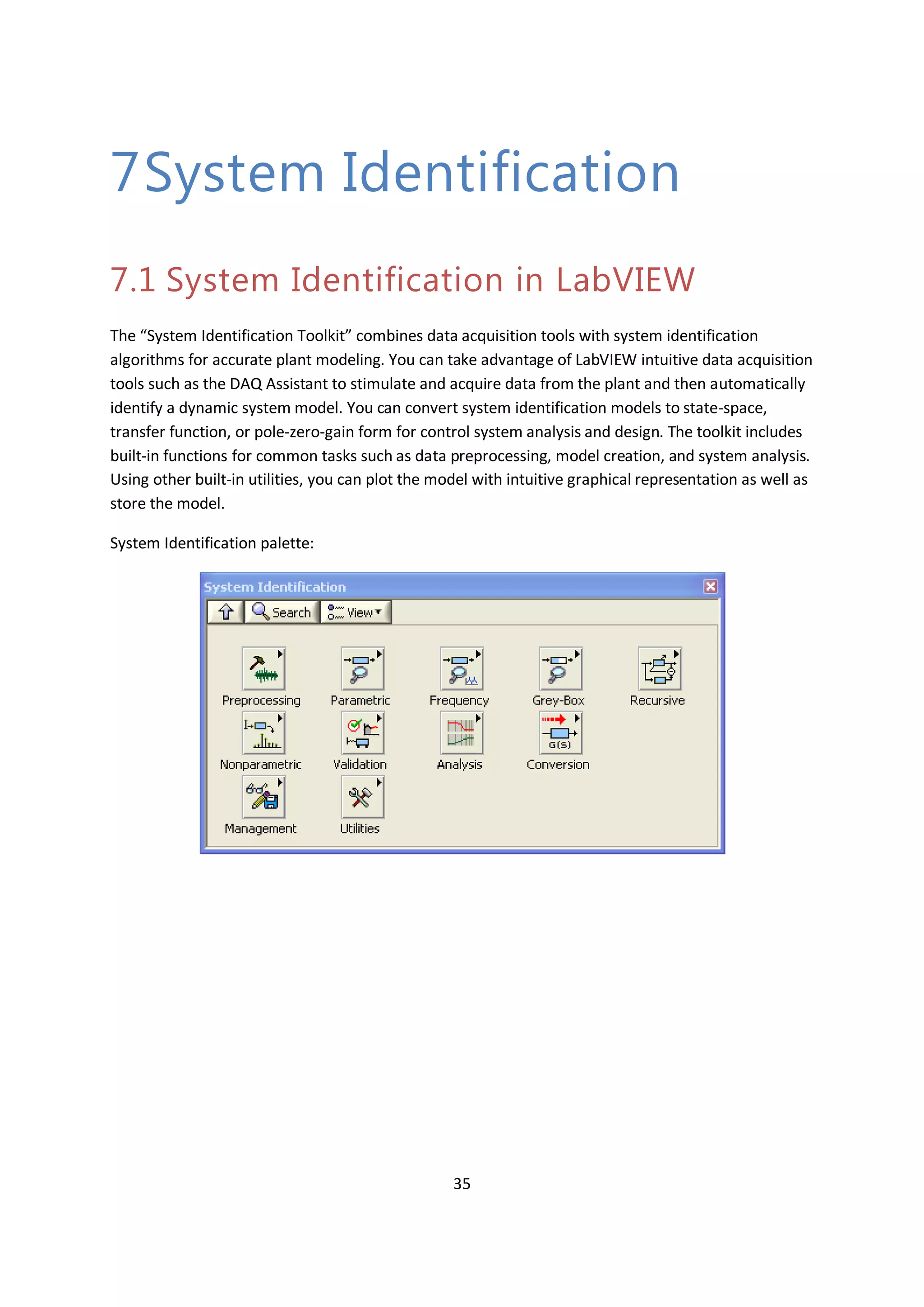
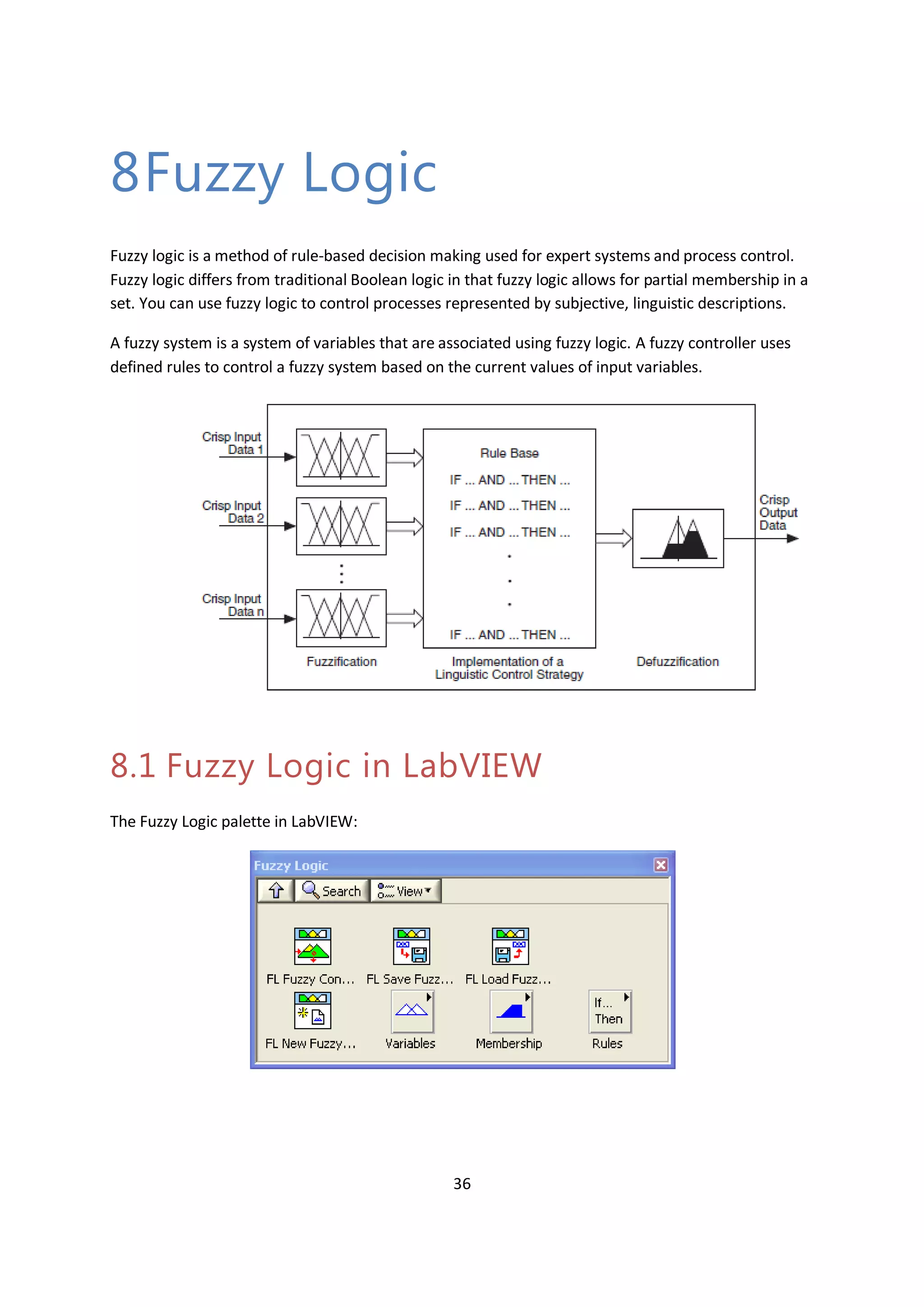
This document provides an introduction to using LabVIEW for control and simulation. It discusses the LabVIEW Control Design and Simulation Module, PID and Fuzzy Logic Toolkit, and System Identification Toolkit. The key aspects of simulation in LabVIEW are covered, including using the Control and Simulation Loop, continuous linear systems functions, and creating simulation subsystems. Examples of simulating a transfer function and spring-mass damper system are provided. Exercises are included to help the reader apply the concepts to modeling and simulating dynamic systems in LabVIEW.