Concrete shrinkage prediction

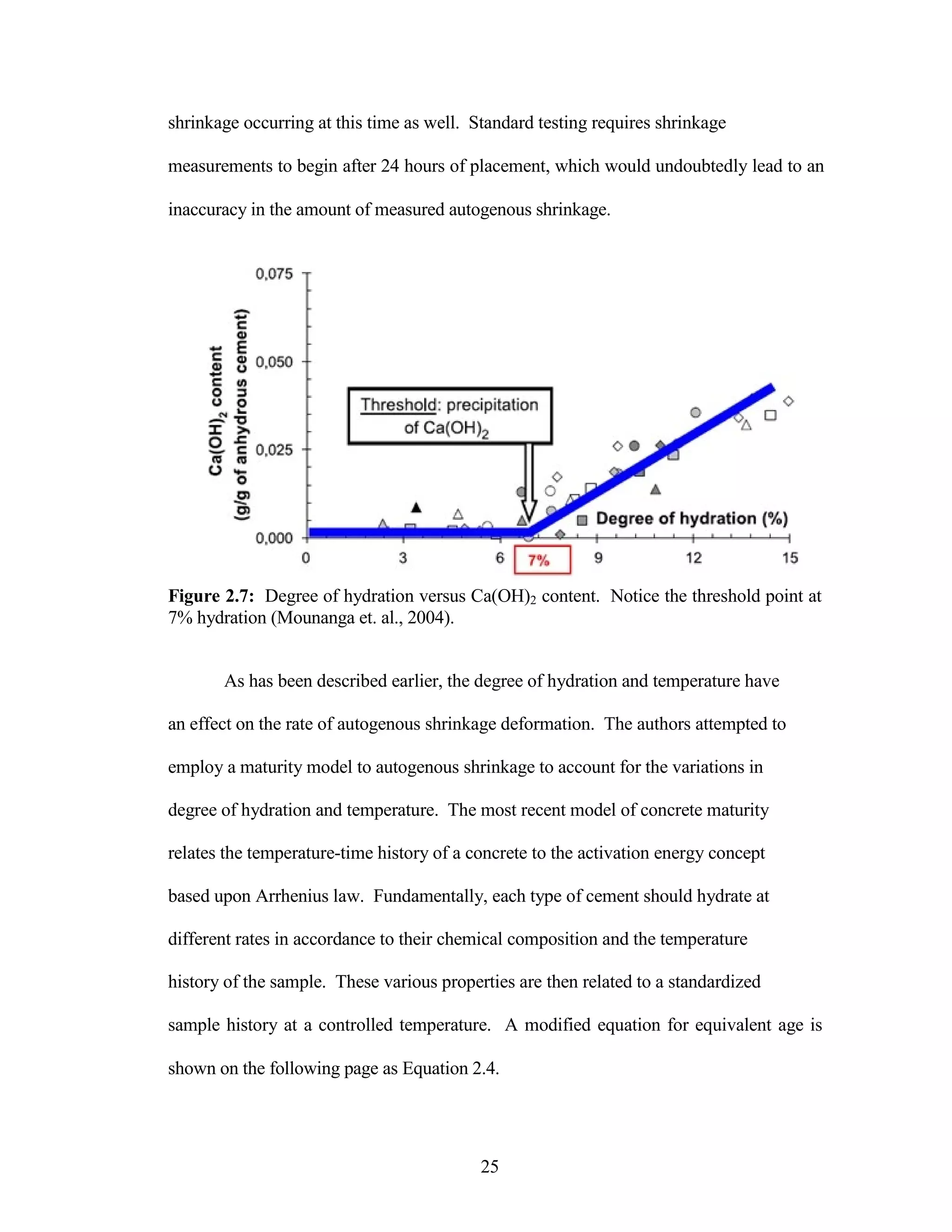
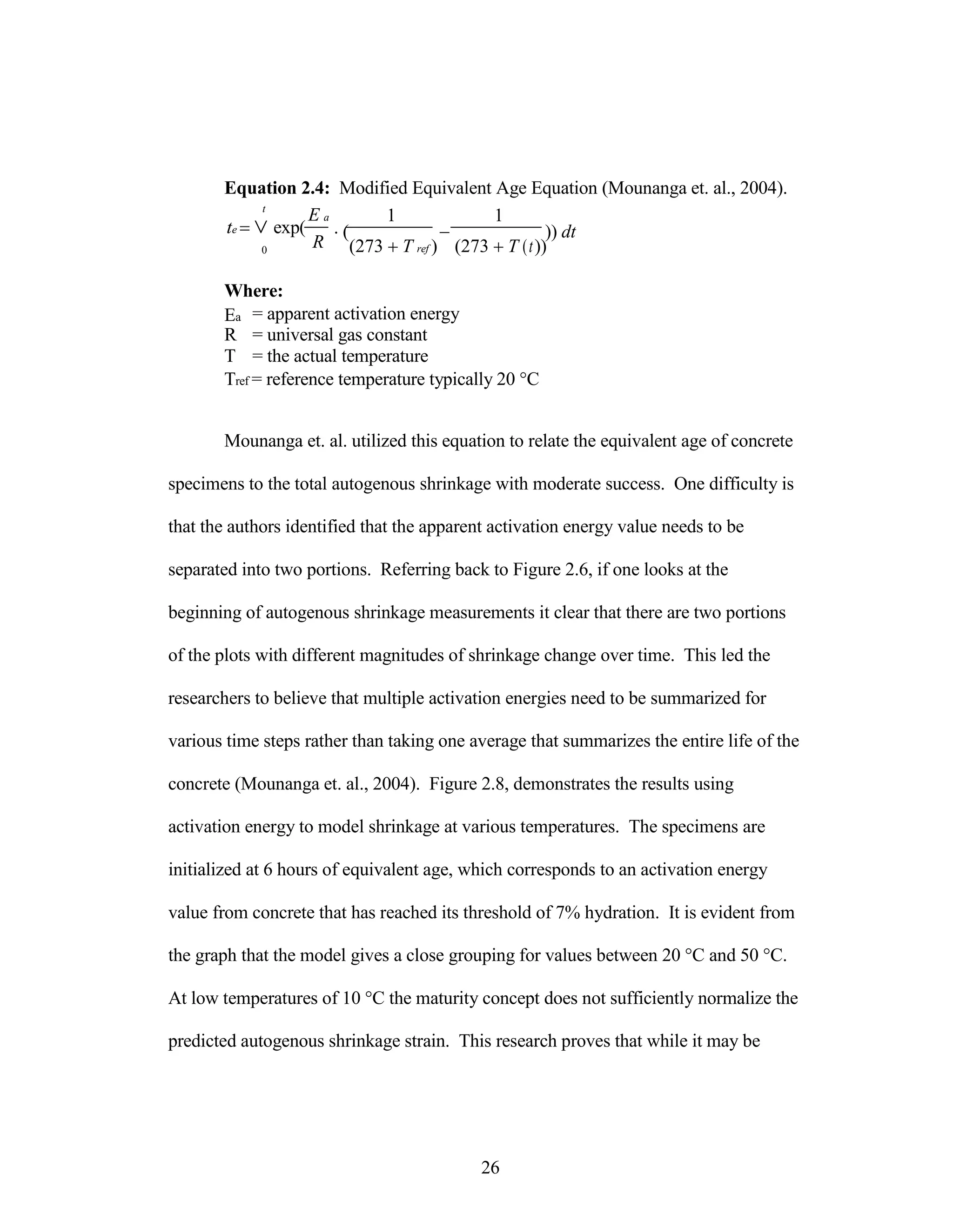
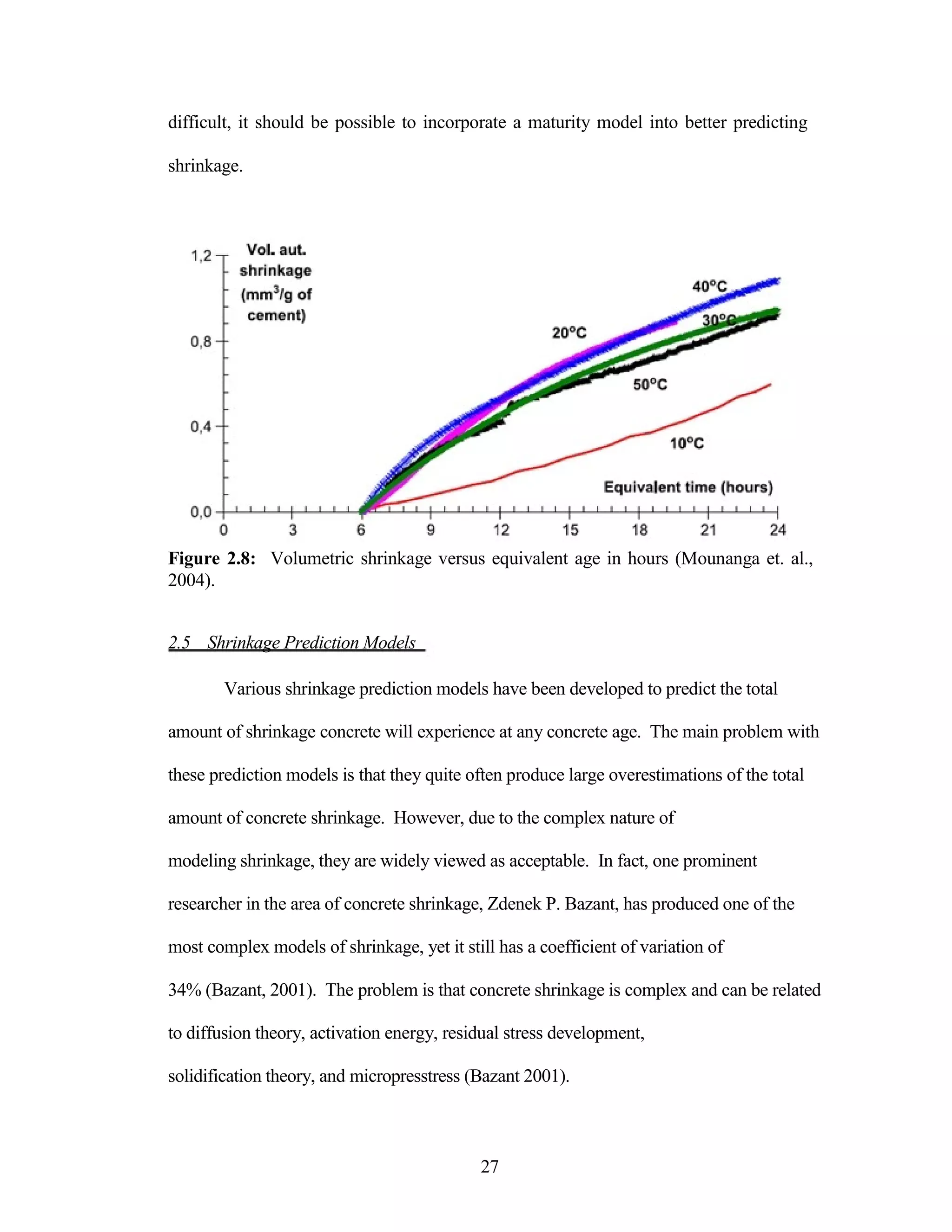
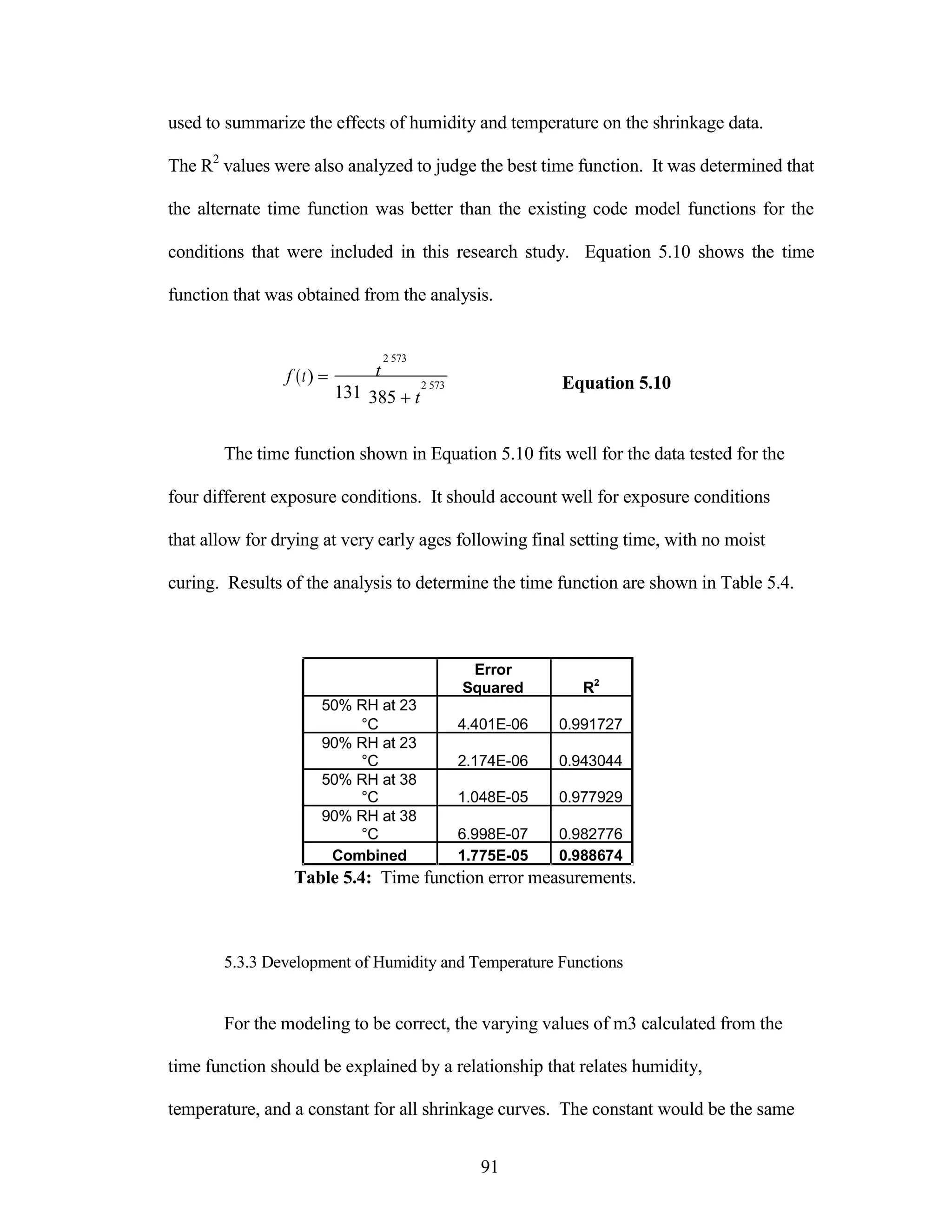
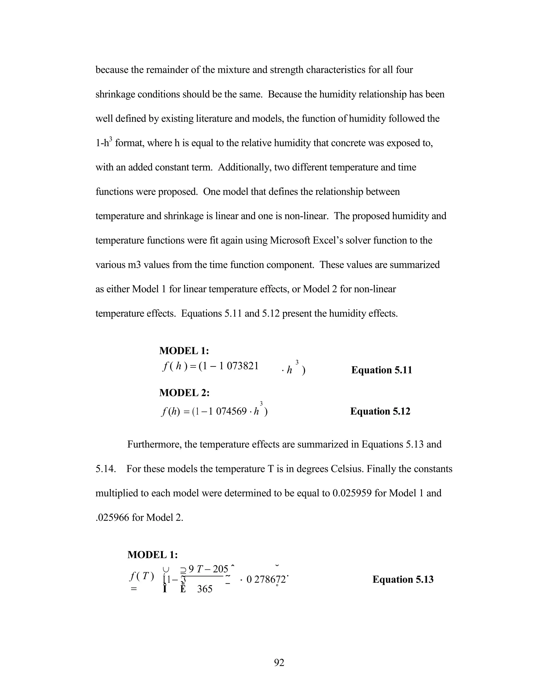
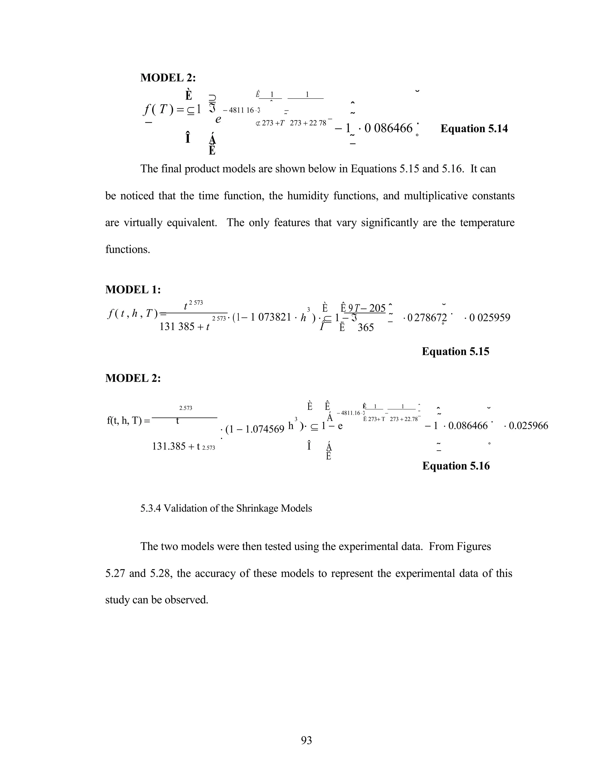
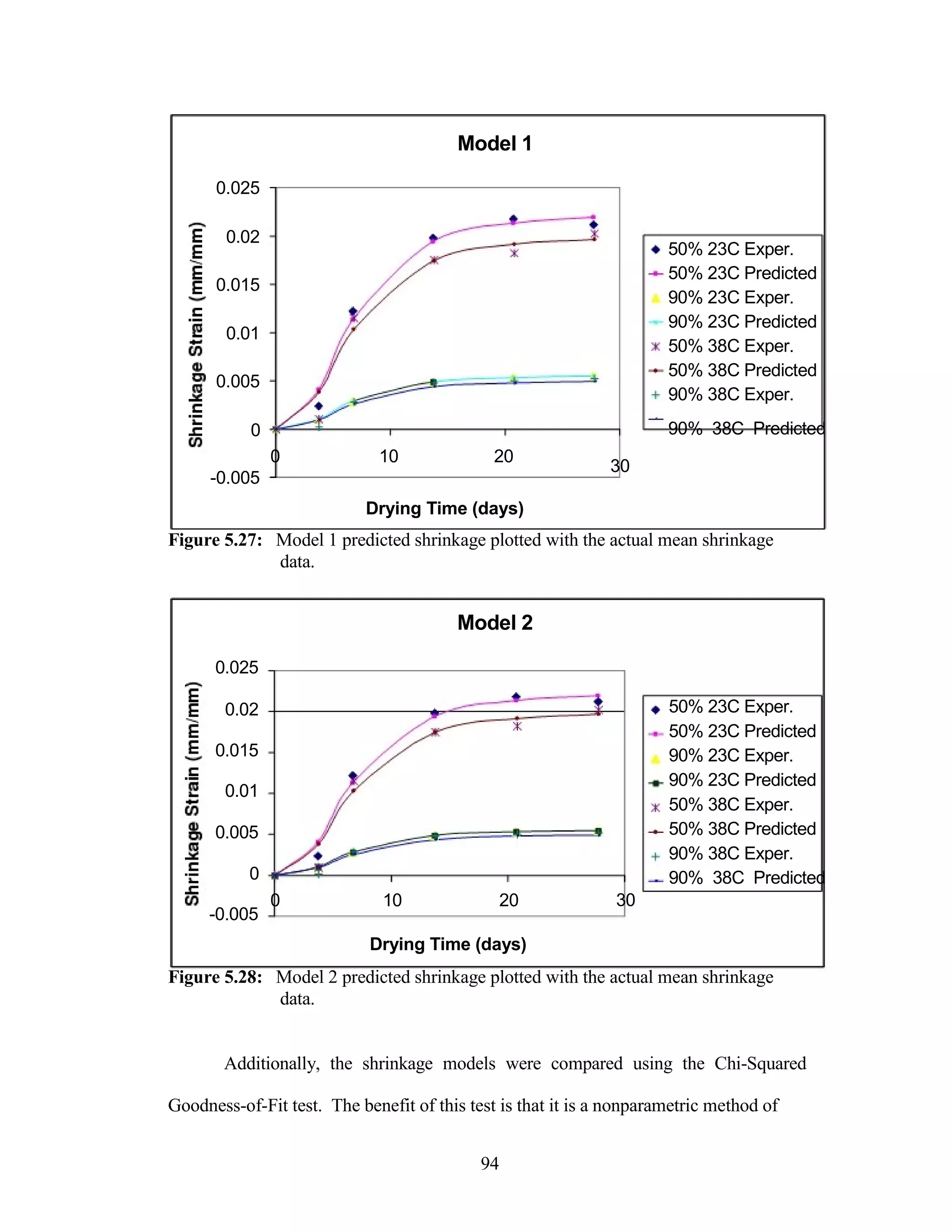
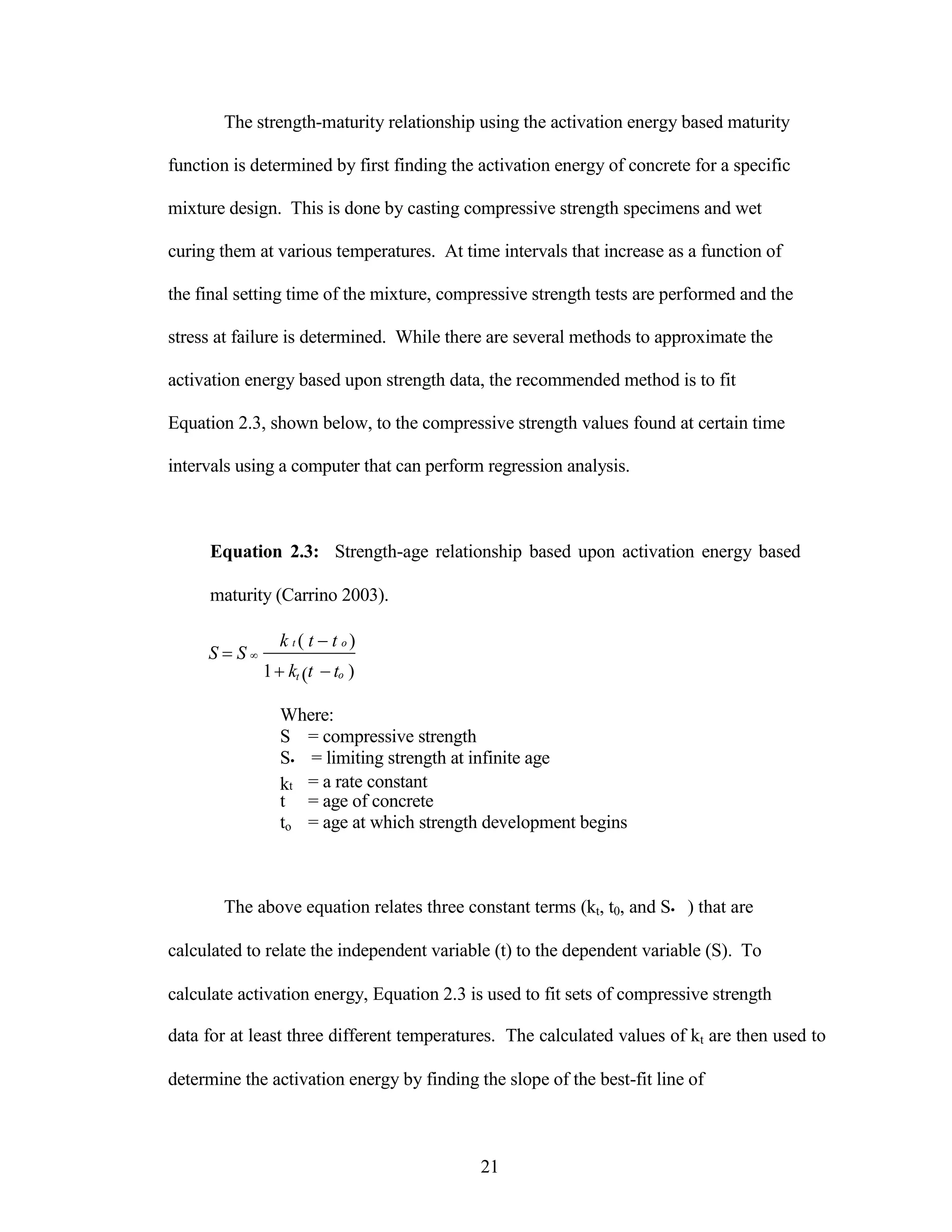
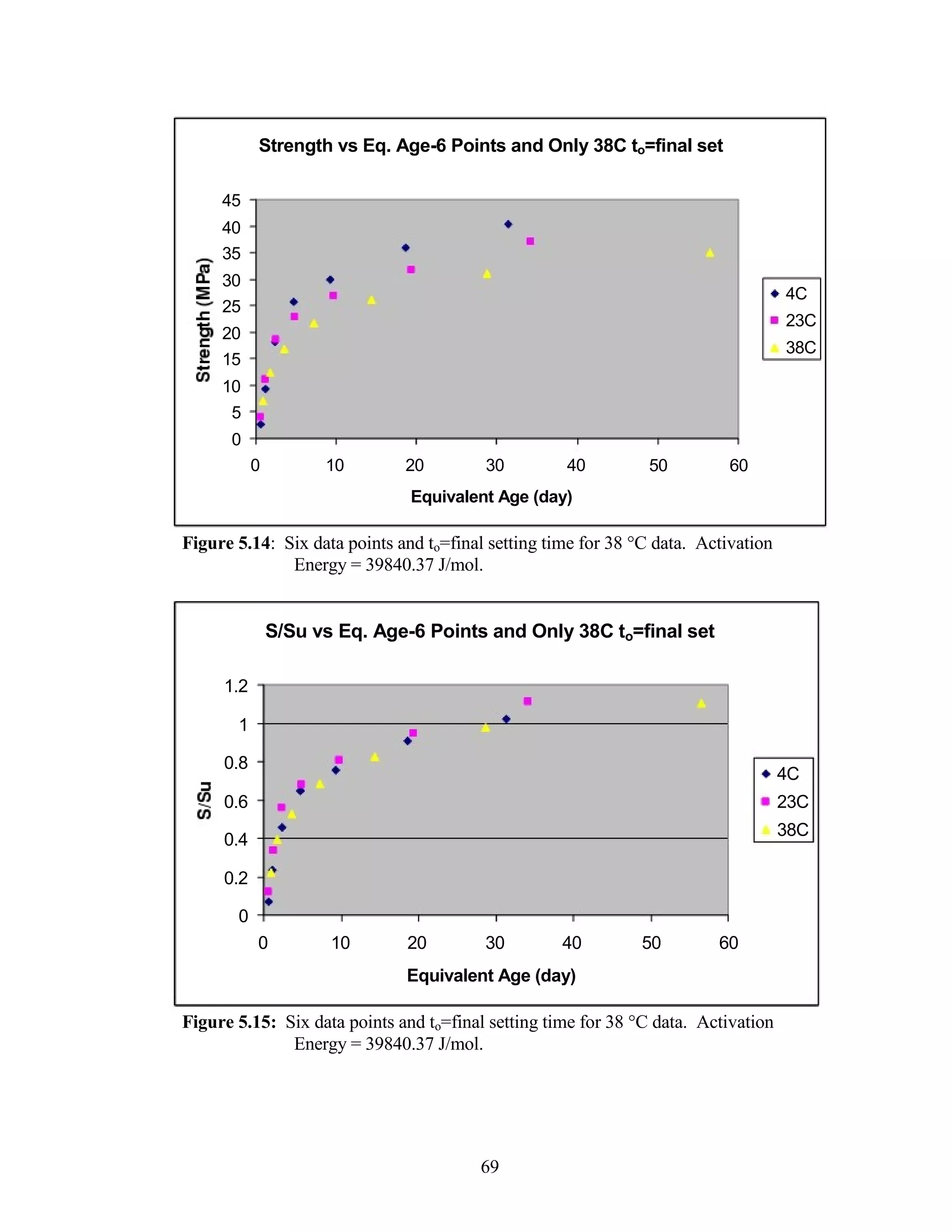
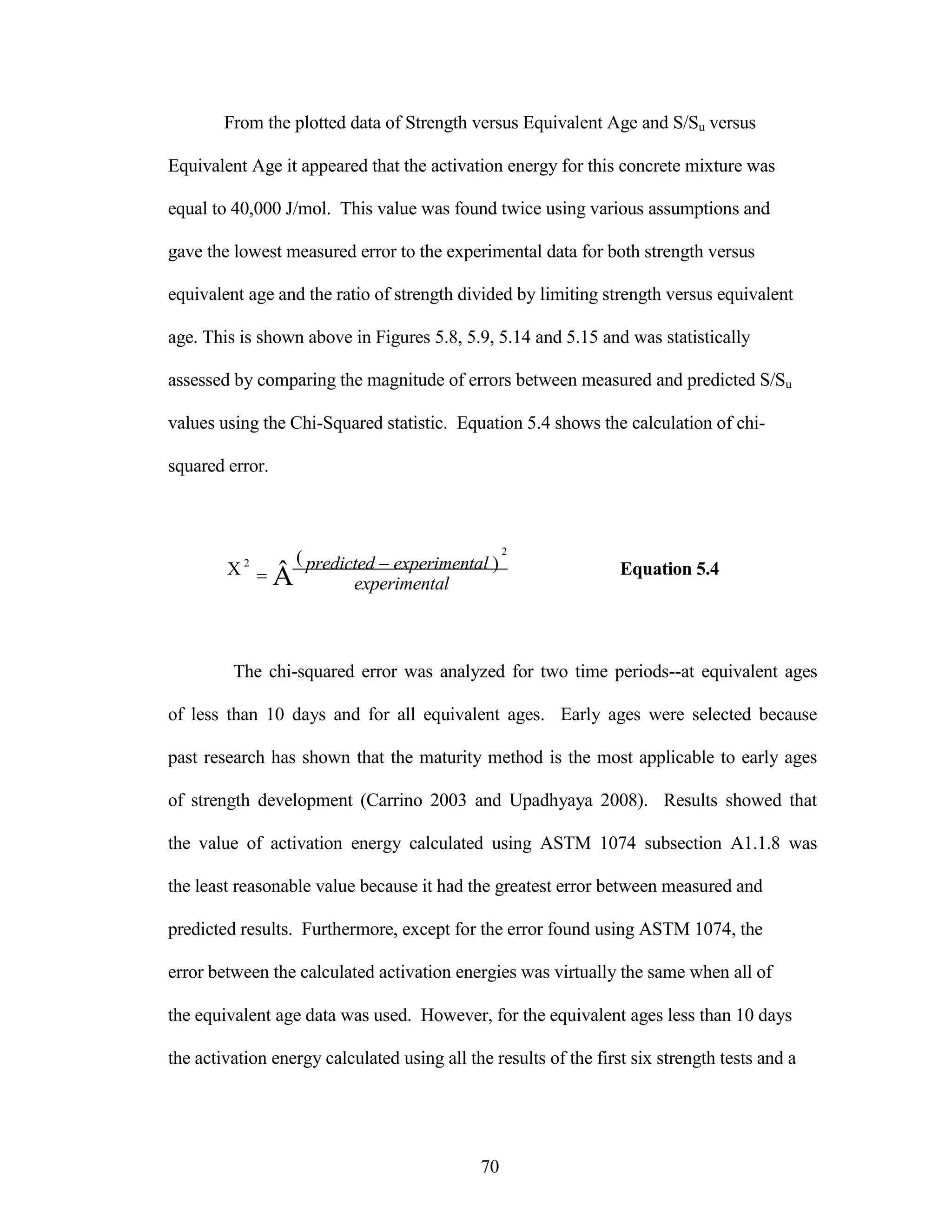
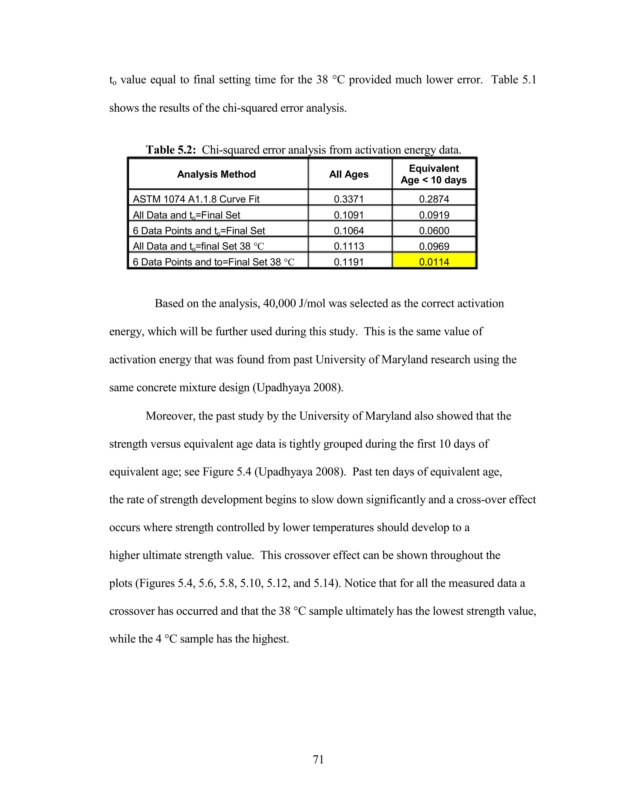
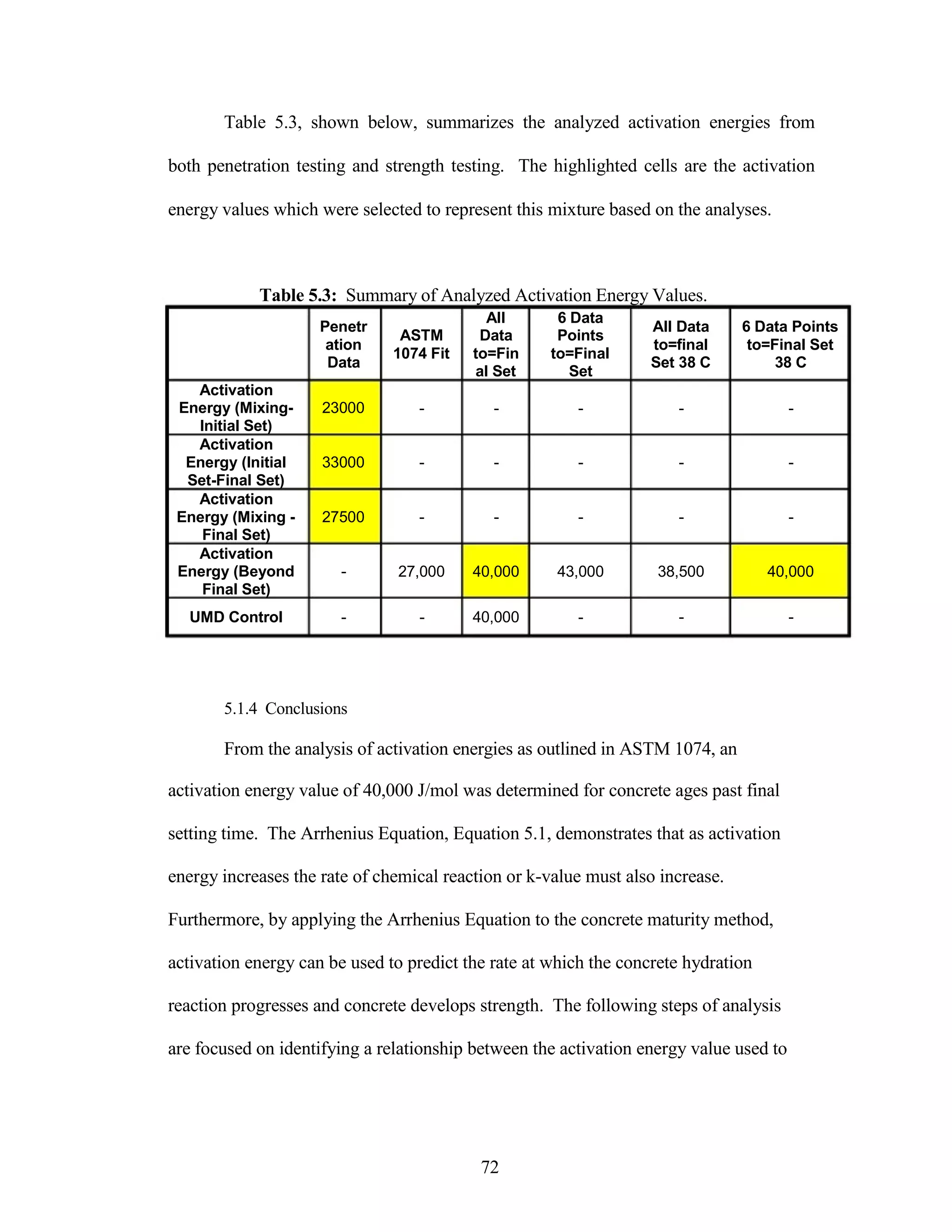
CADmantra Technologies Pvt. Ltd.
Title of Document: CONCRETE SHRINKAGE PREDICTION USING
MATURITY AND ACTIVATION ENERGY
Presented By:Bhola Patel
Design Engineer
CADmantra Technologies Pvt. Ltd.
Contact :bholapatel.me@gmail.com
Shrinkage is a complex material response that often affects concrete in an
adverse manner. The characteristics of the natural environment in which concrete is
placed and the rate of strength development have been used to model the rate of
shrinkage development. Furthermore, concrete maturity has been used to predict the
rate of strength development of concrete cured at different temperatures. This study
sought to find a correlation between activation energy based concrete maturity and
concrete shrinkage. A single concrete mixture was tested to determine the apparent
activation energy of the mixture and the shrinkage under varying environmental
conditions. A shrinkage model incorporating relative humidity and temperature was
developed to predict the shrinkage of the concrete mixture. A relationship between
concrete shrinkage and activation energy based maturity was investigated.

CONCRETE SHRINKAGE PREDICTION USING MATURITY AND
ACTIVATION ENERGY
Table of Contents
Acknowledgements.......................................................................................................... .ii
Table of Contents.......................................................................................................... ...iii
List of Tables ................................................................................................................... . v
List of Figures... ............................................................................................................. .. vi
Chapter 1: Introduction................................................................................................. ... 1
1.1 Introduction.......................................................................................................... .. 1
1.2 Background.......................................................................................................... .. 2
1.3 Research Objectives.............................................................................................. . 3
1.4 Report Organization.............................................................................................. . 4
Chapter 2: Literature Review........................................................................................ ... 5
2.1 Introduction.......................................................................................................... ... 5
2.2 Properties of Concrete Shrinkage ........................................................................ .. 6
2.2.1 Plastic Shrinkage... ....................................................................................... ... 6
2.2.2 Carbonation Shrinkage... .............................................................................. ... 8
2.2.3 Thermal Shrinkage... .................................................................................... ... 9
2.2.4 Autogenous Shrinkage.................................................................................. .. 9
2.2.5 Drying Shrinkage........................................................................................ .. 12
2.3 Concrete Maturity............................................................................................. . 16
2.3.1 Nurse-Saul Method..................................................................................... .. 17
2.3.2 Arrhenius Based Method ........................................................................... ... 20
2.4 Maturity and Shrinkage... ................................................................................ .. 23
2.5 Shrinkage Prediction Models........................................................................... .. 27
2.5.1 ACI 209....................................................................................................... ... 28
2.5.2 CEB-FIP 90... ............................................................................................. ... 30
2.5.3 B3 Model ... ................................................................................................ . 32
2.5.4 GL2000 ...................................................................................................... .. 34
2.6 Performance of Shrinkage Prediction Models................................................ ... 35
Chapter 3: Materials and Testing Plan......................................................................... ... 39
3.1 Materials and Mixture Design ........................................................................... . 39
3.2 Testing Plan ....................................................................................................... .. 42
Chapter 4: Experimental Results ... .............................................................................. .. 45
4.1 Penetration Testing ... .......................................................................................... . 45
4.2 Fresh Concrete Properties.................................................................................. .. 46
4.3 Compressive Strength for Activation Energy Calculations... ........................... .. 47
4.4 Monitoring of Temperatures............................................................................... . 49
4.5 Shrinkage Testing ... .......................................................................................... .. 50
4.6 Compressive Strength Results at Isothermal Conditions................................. ... 52
Chapter 5: Discussion of Results.................................................................................. . 55
5.1 Determination of Activation Energy... ............................................................... .. 55
5.1.1 Penetration Data and Activation Energy Determination ........................... .. 55
5.1.3 Analysis of Calculated Activation Energies ................................................ . 62
5.1.4 Conclusions................................................................................................. .. 72
iii

5.2 Maturity and Shrinkage... ................................................................................. ... 73
5.2.1 Direct Application of Maturity Concept... ................................................... . 73
5.2.2 Maturity Approach as a Function of Ultimate Shrinkage........................... . 77
5.2.3 Derivative Approach to Relate Shrinkage to Activation Energy............... ... 80
5.2.4 Compressive Strength under Shrinkage Curing Conditions..................... ... 83
5.2.5 Conclusions................................................................................................. ... 88
5.3 Shrinkage Modeling........................................................................................... .. 88
5.3.1 Analysis of Existing Shrinkage Models...................................................... .. 88
5.3.2 Development of a Shrinkage Time Function... .......................................... ... 90
5.3.3 Development of Humidity and Temperature Functions ... .......................... . 91
5.3.4 Validation of the Shrinkage Models ............................................................ . 93
5.3.5 Temperature and Humidity Response of Models ....................................... .. 96
5.3.6 Conclusions................................................................................................. ... 99
5.4 Comparison of Model 1 and Model 2 to Existing Models................................. . 99
Chapter 6: Conclusions.............................................................................................. .. 105
6.1 Conclusions....................................................................................................... . 106
6.2 Recommendations.............................................................................................. 107
Appendix A................................................................................................................... 109
References................................................................................................................... .. 114
iv

List of Tables
Table 2.1: Correction Factor for Moist Curing Duration (ACI 209)……………... 29
Table 2.2: Error Percentages and Chi Square Error Percentages for Shrinkage
Models (Mokarem et. al., 2003)…………………………………………………… 36
Table 3.1: Mixture Design and Aggregate Properties…………………………… 40
Table 3.2: Type I/II Portland Cement Physical and Chemical Properties………... 42
Table4.1: Setting Times for 4 °C, 23 °C, and 38 °C…………………………... 46
Table 4.2: Concrete Properties……………………………………………………. 47
Table 4.3: Compressive Strength for 4 °C………………………………………... 48
Table 4.4: Compressive Strength for 23 °C………………………………………. 48
Table 4.5: Compressive Strength for 38 °C………………………………………. 48
Table 4.6: Shrinkage Measurements…………………………………………….... 51
Table 4.7: Compressive Strength Results for Shrinkage Conditioned Samples….. 52
Table 5.1: Calculated Activation Energy Values…………………………………. 62
Table 5.2: Chi-squared Error Analysis of Activation Energy….………………… 71
Table 5.3: Summary of Activation Energy Values………………………………. 72
Table 5.4: Time Function Error Measurements…………………………….……. 91
Table 5.5: Chi-Squared Analysis Results…………………..……………………. 95
Table 5.6: Chi-Squared Values for Existing and Developed Models…….……… 102
Table A.1: Mixture Proportions………………………..…………………………. 109
Table A.2: Consistency data for concrete……………………………………….... 109
Table A.3: Concrete Materials……………………………………………………. 110
Table A.4: Activation Energy-UMD Study (Upadhyaya 2008) …………………. 110
v

List of Figures
Figure 2.1: Plastic Shrinkage Crack Formation (Soroushian and Ravanbakhsh, 1998)
…………………………………………………………………………………….. 8
Figure 2.2: Chemical and autogenous shrinkage behavior (Holt 2001)………….. 12
Figure 2.3: Shrinkage versus Water Content (Videla and Aguilar, 2006)……….. 15
Figure 2.4: Maturity Crossover Effect (Carrino 2003) ………………………….. 19
Figure 2.5: Relative Strength versus Equivalent Age (Carrino 2003)..………….. 23
Figure 2.6: Autogenous Shrinkage versus Concrete Age (Mounanga et. al., 2004)
…………………………………………………………………………………….. 24
Figure 2.7: Degree of Hydration versus Ca(OH)2 Content (Mounanga et. al., 2004)
…………………………………………………………………………………….. 25
Figure 2.8: Volumetric Shrinkage versus Equivalent Age (Mounanga et. al., 2004)
…………………………………………………………………………………….. 27
Figure 2.9: Shrinkage versus age (Goel et. al., 2007)..………………………….. 38
Figure 3.1: Coarse Aggregate Gradation..……………………………………….. 41
Figure 3.2: Fine Aggregate Gradation.………………………………………….. 41
Figure 3.3: Aggregate Blend Gradation…..…………………………………….. 42
Figure 4.1: Penetration Testing Results ..……………………………………….. 46
Figure 4.2: Activation Energy Compressive Strength Testing Results………….. 49
vi

Figure 4.3: Monitoring of Isothermal Conditions…….………………………….. 50
Figure 4.4: Shrinkage Results…………………………………………………….. 52
Figure 4.5: Compressive Strength -Conditioned Samples……………………….. 53
Figure 4.6: Compressive Strength-Conditioned Samples at Early Ages…..…….. 53
Figure 5.1: AE Determination Based Upon Penetration Data-Mixing to Initial
Set………………………………………………………………………………….. 56
Figure 5.2 AE Determination Based Upon Penetration Data-Mixing to Final
Set………………………………………………………………………………….. 57
Figure 5.3: AE Determination Based Upon Penetration Data-Initial Set to Final
Set………………………………………………………………………………….. 57
Figure 5.4: S vs. Equivalent Age-Control (Upadhyaya 2008)……………………. 63
Figure 5.5: S/Su versus Equivalent Age-Control (Upadhyaya 2008) ……………. 64
Figure 5.6: S vs. Equivalent Age-ASTM 1074-A1.1.8…….…..………………… 65
Figure 5.7: S/Su versus Equivalent Age-ASTM 1074-A1.1.8..………………….. 65
Figure 5.8: S vs. Equivalent Age-All Data with to = final setting time………….. 66
Figure 5.9: S/Su versus Equivalent Age-All Data with to = final setting time..….. 66
Figure 5.10: S vs. Equivalent Age-Six data points and to = final setting time..…. 67
vii

Figure 5.11: S/Su versus Equivalent Age-Six data points and to = final setting
time………………………………………………………………………………… 67
Figure 5.12: S vs. Equivalent Age-All data with to = final setting for 38 °C
data…………………………………………………………………………………. 68
Figure 5.13: S/Su versus Equivalent Age-All data with to = final setting for 38 °C
data………………………………………………………………………..……….. 68
Figure 5.14: S vs. Equivalent Age-Six data points and to=final setting time for 38 °C
data……………………………………………………………………..………….. 69
Figure 5.15: S/Su versus Equivalent Age-Six data points and to=final setting time for
38 °C data…..………………………………..…………………………………….. 69
Figure 5.16: Shrinkage versus Actual Concrete Age…………………………….. 74
Figure 5.17: Shrinkage versus Equivalent Age……….………………………….. 75
Figure 5.18: Shrinkage versus Age Divided by the Age Conversion Factor…….. 76
Figure 5.19: e/eu versus Equivalent Age ………..……………………………….. 78
Figure 5.20: e/eu versus Age Divided by Age Conversion Factor….…………….. 79
Figure 5.21: e/eu versus Age... .……………………………………………….. 80
Figure 5.22: Derivative of the Shrinkage Polynomial versus Time …….……….. 82
Figure 5.23: Earlier age Compressive Strength Development versus Time………. 84
Figure 5.24: Compressive Strength of Conditioned Samples versus Equivalent
Age…………………………………………………………………………………. 85
Figure 5.25: Shrinkage versus Compressive Strength-50% RH….……………….. 86
viii

Figure 5.26: Shrinkage versus Compressive Strength -90% RH………………….. 86
Figure 5.27: Model 1 Predicted Shrinkage and Experimental Shrinkage………….94
Figure 5.28: Model 2 Predicted Shrinkage and Experimental Shrinkage……….. 94
Figure 5.29: Humidity Response of Model 1…………………………………… 97
Figure 5.30: Temperature Response of Model 1……………………………….. 97
Figure 5.31: Humidity Response of Model 2…………………………………… 98
Figure 5.32 Temperature Response of Model 2………………………………… 98
Figure 5.33: Shrinkage Data (50% RH at 23˚C) and Existing and Developed
Models……………………………………………………………………………... 100
Figure 5.34: Shrinkage Data (90% RH at 23˚C) and Existing and Developed
Models……………………………………………………………………………... 101
Figure 5.35: Percentage Residual Error-50% RH at 23˚C………………………..103
Figure 5.36: Percentage Residual Error-90% RH at 23˚C………………………. 103
Figure 5.37: Percentage Residual Error-50% RH at 38 ˚C……………………… 104
Figure 5.38: Percentage Residual Error-90% RH at 38 ˚C……………………… 104
ix

Chapter 1: Introduction
1.1 Introduction
Many materials used for civil engineering applications are impacted by
changes in environmental factors, manufacturing practices, and composition
characteristics. Asphalt, for instance, changes its stiffness characteristics as its
temperature increases or decreases. Furthermore, a seemingly uniform material such
as steel can possess a wide array of characteristics by varying elements such as
carbon content or by applying different heat treatments during manufacturing. Even
natural products such as timber can possess different strength characteristics if kept
moist rather than dry. Portland cement concrete is also impacted by similar
characteristics. Environmental factors, mixture design, placement, and curing
characteristics significantly affect the rate and degree of strength development, as
well as the durability, of concrete. Achieving an understanding of these
characteristics and how they affect concrete is a significantly challenging and
fulfilling task.
Concrete shrinkage is a physical response that concrete displays due to many
different parameters. These include water-to-cement ratio, coarse and fine aggregate
proportions, percentage of exposed surface area, cement type, compressive strength,
curing temperature and humidity, and exposure time. Since the beginning of the
twentieth century, engineers and scientists have attempted to identify the variables
that cause shrinkage and to develop a methodology to predict shrinkage. Shrinkage
1

prediction has proven to be difficult to accurately assess because many of the
variables that affect concrete shrinkage are complexly related to one another.
The fundamental problem with shrinkage is that it can cause undesirable stress
development in concrete which can lead to cracking. Cracking, in turn, will lead to a
reduction in strength and durability. If the degree of strain developed by concrete
shrinkage could be accurately predicted, then it is possible that the detrimental effects
of strength and durability reduction could be minimized and accounted for with better
designs.
1.2 Background
As previously stated, concrete shrinkage is a difficult material behavior to
predict because of the many factors affecting this property. In general, however,
concrete shrinkage is a result of the development of negative pore pressures within
concrete. Since the development of negative pore pressure can occur in several
different ways and at different concrete ages, engineers have characterized concrete
shrinkage by five different types: plastic shrinkage, autogenous shrinkage, thermal
shrinkage, carbonation shrinkage, and drying shrinkage. The sum of these five types of
shrinkage equals total shrinkage. It is common for drying shrinkage to simply be referred
to as shrinkage because the majority of the measurable volumetric change, when compared
to the other forms, is due to drying.
Furthermore, concrete shrinkage has been found to be related to the magnitude
of developed concrete strength as well as the rate at which concrete strength develops.
In fact, several researchers have looked at both autogenous and chemical shrinkage
and found that they are proportional to the rate at which concrete strength develops
2

through hydration (Mounanga et. al 2004). In turn, they have utilized activation
energy based concrete maturity to build this relationship for chemical and autogenous
shrinkage. The maturity function relates how rapidly concrete gains strength at
different temperatures in relation to the chemical reaction known as hydration. This
maturity relationship can then be applied to various temperatures to accurately predict
concrete strength with age. Using this existing knowledge, it seems plausible that
total shrinkage could be better predicted by incorporating concrete maturity into
shrinkage modeling.
1.3 Research Objectives
The primary objective of this investigation was to determine whether a link between
the total amount of concrete shrinkage (experienced at different
temperatures) and concrete maturity (based upon activation energy) existed. French cement
researchers have demonstrated a relationship between chemical and
autogenous shrinkage during the early ages of concrete strength development while concrete
is still semi-rigid. It would be a valuable improvement to show that concrete maturity can be
related to the total amount of shrinkage, rather than simply to some components of shrinkage
such as chemical shrinkage.
To achieve this objective, this research investigation was broken into several
different objectives which are listed as follows:
1. to determine the setting times of concrete and use this information to
calculate activation energies for time periods at early ages, prior to final
setting time;
3

2. to determine the activation energy at later ages using strength data from
different temperature exposures;
3. to measure and compare shrinkage at different temperatures and
relative humidity levels;
4. to establish a relationship between concrete maturity (based upon
activation energy) and concrete shrinkage;
5. to develop a model that predicts the concrete shrinkage as a function of
the temperature and humidity levels;
6. to compare existing shrinkage prediction models to the model
developed by this study to assess its validity.
1.4 Report Organization
The first chapter of this thesis contains the introduction, research objectives, a
brief description of the background, and the organization of the report. The following
chapter reviews the existing literature to comprehensively summarize the state of
knowledge on concrete shrinkage and concrete maturity. The third chapter presents
the testing plan and the materials used. Next, the fourth chapter presents the
experimental results from the laboratory testing. The fifth chapter presents the
analysis of the data including results of the activation energy calculations, shrinkage
and maturity correlation, shrinkage modeling, and model comparison. The sixth and
final chapter summarizes the research work, draws conclusions based upon this work,
and provides recommendations for further improving concrete shrinkage predictions.
4

Chapter 2: Literature Review
2.1 Introduction
It is well known that concrete is a heterogeneous material composed of
various sized aggregates, cementitcious materials, water, and a multitude of
admixtures and additives. Understandably, it is difficult to completely predict and
model the long term behavior of concrete with such non-uniformity found in its
components. As concrete ages it tends to reduce in volume. This phenomenon is
known as shrinkage, and is typically related to a loss of water from concrete over
time, but can also be associated with environmental exposure and temperature.
Researchers have attempted to model the behavior of shrinkage and concrete creep,
but as described by Bazant, “…shrinkage is still far from being fully understood, even
though it has occupied some of the best minds in the field on cement and concrete
research and materials science (Bazant 2001).” However, researchers do seem to
have a good grasp of the mechanisms driving the volume change of concrete.
Each of these mechanisms has been defined as its own type of shrinkage and
broken into components of a complete volume change known as total shrinkage.
These various components include plastic shrinkage, drying shrinkage, autogenous
shrinkage, thermal shrinkage, and carbonation shrinkage. One of the difficulties in
predicting total shrinkage is that each of these components of concrete shrinkage has
its own driving factors which can create an immense number of variables to
5

incorporate into prediction models. Therefore, many researchers attempt to simplify
their calculations by only observing autogenous shrinkage and drying shrinkage as
substitute for total shrinkage because their magnitudes will be greater than other types
of shrinkage. Thermal shrinkage is accurately described as thermal expansion and
contraction of concrete due to temperature change, and can be reversed upon heating;
therefore, it will not be discussed as a contributing shrinkage mechanism.
It is important to understand and to be able to predict the amount of shrinkage,
because the strain that occurs will translate into stress development and cracking
within a concrete section. The degree of shrinkage will be much greater at early ages.
It has been shown from research that concrete sections will typically display
approximately 50% of its total shrinkage within the first 28 days of drying and 80%
within the first 90 days of drying (Altoubat and Lange, 2001). The problem with
significant early shrinkage is that concrete at early ages may not have developed
sufficient rigidity and strength to resist the tensile stresses developed by shrinkage.
Properly predicting these stresses could lead engineers to better predict whether or not
cracking will be acceptable, what mixture components can be modified to account for
shrinkage, and what curing techniques could be used to minimize shrinkage.
2.2 Properties of Concrete Shrinkage
2.2.1 Plastic Shrinkage
Chronologically, plastic shrinkage occurs before all other types of shrinkage,
and therefore, it will be discussed first. Plastic shrinkage is defined as the volume
change of concrete associated with water lost while concrete is still in a plastic state
(Aitcin et. al., 1997). When water is removed from concrete paste while still in a
6

plastic state, a series of menisci are formed which generate negative capillary
pressures that cause volume contraction of the paste. These pressures will continue to
rise until enough pressure is reached that the water will begin to rearrange within the
paste such that it pools and forms voids. This process can be attributed to the loss of
water from the surface or subgrade of concrete. Often, the surface of the concrete
will begin to dry and attain some initial rigidity before any other portion of the
concrete structure and will no longer undergo plastic flow. This proves to be
problematic, because it leads to the formation of plastic shrinkage cracking, which
typically act as pathways for moisture to exit the concrete system. Figure 2.1
demonstrates the mechanisms driving the formation of plastic shrinkage cracks.
Notice that the surface is dry while the base is moist, which is integral to forming
shrinkage cracks; clearly if it was still somewhat fluid the shrinkage cracks would not
form. Plastic shrinkage cracking can be significantly reduced, if not completely
eliminated, simply by providing adequate moisture to the concrete through good
curing practices.
7

Figure 2.1: Plastic Shrinkage Crack Formation (Soroushian and Ravanbakhsh,
1998).
2.2.2 Carbonation Shrinkage
Another form of shrinkage, which occurs after the final setting of concrete, is
carbonation shrinkage. By definition, carbonation shrinkage is caused by a chemical
reaction between the hydrated cement paste and carbon dioxide found in air (Aitcin
et. al., 1997). The carbonation reaction occurs between the calcium hydroxide
molecules (Ca(OH)2) and Carbon Dioxide (CO2) found in air under the presence of
moisture. Clearly, the degree of carbonation shrinkage is dependent upon how
permeable to air is the concrete specimen. This in turn means that concrete that is
well cured and has a low water-to-cementitcious material ratio will undergo less
carbonation shrinkage as it ages.
The amount of carbonation shrinkage that occurs is typically at a maximum at
relative humidity around 50%, while its amount is negligible at relative humidity below
25% or above 100%. It has been stated by Powers that carbonation shrinkage results from
the dissolution of calcium hydroxide crystals which are under
8

compression due to the drying shrinkage, leading to the formation of stress-free
calcium carbonate in the pores (Powers 1962). This means that the effects of drying
shrinkage and carbonation shrinkage are correlated. Once the carbonation process
begins, it causes the pore voids to densify and realign to a lower stress state. This
helps explain why drying shrinkage specimens, when rewetted, may not return to the
original volume prior to drying. The carbonation shrinkage reduces the amount of
water that can be reabsorbed.
2.2.3 Thermal Shrinkage
Thermal shrinkage is a reaction by the concrete to a reduction of temperature
shortly after the formation of a rigid concrete structure. During the chemical
hydration reaction there is an inevitable increase in the temperature of concrete
because the reaction itself is an exothermic reaction. Following the peak of this
reaction, heat is dissipated causing a cooling of the concrete structure and a volume
reduction as a result of this cooling. Some researchers believe that this cooling
behavior would be more accurately described as thermal contraction rather than
thermal shrinkage (Aitcin et. al., 1997). Thermal shrinkage is due solely to the
thermal expansion and contraction coefficients rather than the buildup of negative
pore pressures, as in the four other types of shrinkage. However, like the other types
of shrinkage formation the concurrent volume reduction can lead to cracking and
other problems. Thermal shrinkage would be most pronounced in large concrete
mass structures that can generate a significant amount of heat during hydration.
2.2.4 Autogenous Shrinkage
Autogenous shrinkage is a phenomenon that is almost mysterious when producing
concrete. This is because there can be a volume change found in concrete even
9

within sealed specimens free of environmental effects. Autogenous shrinkage is
defined as the macroscopic volume reduction of cementitcious materials when cement
hydrates after initial setting. This type of shrinkage can also be referred to as self-
desiccation shrinkage, because within the concrete macroscopic pore structure as
water hydrates with cement particles to produce hydrated cement paste, the water and
cement reduce in volume. This reduction in volume develops negative pressures
within the capillary pores. The major problem is that concrete at an early age has
minimal strength; in fact, autogenous shrinkage tends to plateau as the degree of
concrete hydration reduces typically after 24 hours (Mounanga et. al., 2004). This
means while capillary pressures developed due to cement hydration may be small,
these pressures can still produce measurable shrinkage values.
Furthermore, autogenous shrinkage can often be confused with what is called
chemical shrinkage. To clarify the variation, chemical shrinkage is a result of the
reaction occurring between water and cement causing a reduction in the volume of
the hydrated byproduct. Chemical shrinkage is often measured by sealing a cement
paste specimen in an impermeable membrane and placing it in a water bath under a
weigh below scale to see what the reduction in the upward buoyancy force is over
time. As the sealed mass would remain constant, any reduction in volume would
cause an increase in measured mass because the cement paste would have less
displaced volume of water. This means that chemical shrinkage is a measured total
volume change which may prove to cause no measurable external dimensional
change.
10

Autogenous shrinkage, however, is the externally measurable reduction in
volume. In fact, researchers have explained that autogenous shrinkage has three
different phases of formation (Holt 2001). First is the liquid stage where the material
is still highly fluid and has not formed its structure. Autogenous shrinkage during
this phase is the same as the measured chemical shrinkage. Second is the skeleton
formation phase, where the concrete is semi-rigid and autogenous shrinkage is a
function of both self desiccation as well as chemical shrinkage. During this phase the
measured autogenous shrinkage will begin to diverge from the measured chemical
shrinkage, as shown in Figure 2.2. Finally, autogenous shrinkage reaches the
hardened phase, when the concrete is rigid and chemical shrinkage will have little to
no effect on the measured autogenous shrinkage but rather the self desiccation of the
internal relative humidity within the concrete will cause the measurable volume
change.
11

Figure 2.2: Chemical and autogenous shrinkage behavior over time.
Note: Notice that at early ages the two shrinkages are proportional, but at later ages they
diverge significantly (Holt 2001).
Traditionally, autogenous shrinkage has been neglected from consideration in
measurements of total shrinkage. This is because at normal range water-to-cement
ratios, the magnitude of autogenous shrinkage is very small in comparison to drying
shrinkage measurements. However, with the advent of high-performance concrete
(HPC), which has low water-to-cement ratios, autogenous shrinkage strains are as or
more significant than drying shrinkage strains (Aiticin 1999). It has been shown that
water-to-cement ratios below 0.33 typically will produce significant amounts of
autogenous shrinkage strains.
2.2.5 Drying Shrinkage
Drying shrinkage is the most commonly recognized form of shrinkage.
Drying shrinkage is caused by the development of capillary tension, solid surface
12

tension, and withdrawal of hindered absorbed and interlayer water from cement gel
(Bazant 2001). The definition for drying shrinkage is the reduction in volume due to the
effect of moisture loss from environmental exposure after concrete has set.
Effectively, this is the drying of the moisture found in the pores on the surface of the
exposed concrete. Clearly, this means that concrete dimensions can play a large roll in the
degree of drying shrinkage that occurs; more exposed surface area will lead to a greater
amount of shrinkage.
Due to the significant effect that concrete drying shrinkage has on the total
shrinkage concrete will experience, Chilean researchers Videla and Aguilar looked at
the drying shrinkage of blended and normal Portland cement concretes. They
developed a comprehensive study where they sought to minimize the amount of
drying shrinkage by optimizing the mixture design components. Their study
effectively broke down testing into two phases. The first phase looked at the effects
of the mixture design variables on drying shrinkage by varying the type of aggregate,
the nominal maximum aggregate size, the slump achieved, and the type and blend of
cement with varying finenesses. The second phase of the study was designed to
isolate the effects of cement on drying shrinkage by varying the type of cement and
cement content. In turn, the aggregate type, slump, and nominal maximum aggregate
size were kept constant (Videla and Aguilar, 2006). It is important to note that they
used their national naming system for describing the types of cement used. These
included Portland cement (P similar to Type III), coarse Portland pozzolan cement
(PPC, a slow hardening cement), and fine Portland Pozzolan Cement (PPF, a fast
hardening cement).
13

In discussion of the results it was shown through an analysis of variance test
(ANOVA) that the researchers attempted to identify significant independent variables
affecting drying shrinkage. It was shown that for concretes with equal compressive
strength, the relevance of the independent variables on drying shrinkage in order of
importance is: drying time, volume-to-surface ratio, cement type, aggregate
maximum size, aggregate type, cement type to aggregate type, and aggregate type to
volume-to-surface ratio (Videla and Aguilar, 2006). Furthermore, Figure 2.3 shows
that with increasing water content the magnitude of drying shrinkage experienced
also increases. This proves to be constant for various drying times. This can be
explained by the fact that concrete with a lower water-cement ratio will produce
concrete with lower permeability and therefore less ability for capillary pores to dry
over time.
14

Figure2.3: Observed drying shrinkage versus the water content for two different time
periods, 56 days and 720 days.
Note: S corresponds to siliceous aggregate and L corresponds to limestone
aggregate. Notice that as water content is increasing amount of drying shrinkage
appears to increase (Videla and Aguilar, 2006).
Interestingly, it was shown that even though limestone aggregate requires
more water content to achieve a desired slump than siliceous aggregates, it displays
less drying shrinkage over time. Videla and Aguilar propose that this is because the
limestone aggregate used has a higher modulus of elasticity than the siliceous
aggregate used (Videla and Aguilar, 2006). Moreover, it has been suggested that the
amount of drying shrinkage that occurs is influenced by the aggregate content in
concrete, meaning that more or less aggregate by volume of a cubic yard of concrete
will effect drying shrinkage. This was proven by the results from Videla and Aguilar
and led them to conclude that the amount of drying shrinkage can be reduced by
using an aggregate with a high elastic modulus and in large amounts (Videla and
Aguilar, 2006).
15

The results of the second portion of their study looked at the effects of various
types of Portland cement on drying shrinkage. However, the results of their analysis
prove to be difficult to interpret since the cement types used do not follow standard
ASTM nomenclature. What was uncovered was that the cement type that had the
highest degree of shrinkage was the coarse grained Portland pozzolan cement (PPC).
The fine grained Portland pozzolan cement (PPF) had less drying shrinkage than type
PPC but more than the Portland cement (P) (Videla and Aguilar, 2006). What this
can be interpreted as meaning is that the coarse grained cements, PPC, should hydrate
more slowly and be more susceptible to volume changes than the faster hydrating
type PPF and P cements. This makes sense, if one considers that the PPC concrete
should have a slower strength gain over time versus the other types, which in turn
means that its elastic modulus will be lower.
2.3 Concrete Maturity
Concrete exhibits a relationship between strength development and
temperature. As the temperature of concrete increases, its rate of strength gain
increases and vice versa. This can prove to be problematic when trying to predict whether
or not a certain sample of concrete has achieved adequate strength
development for the loading it will endure. A standard relationship needed to be
developed so that the daily variation in temperature could be accounted for in
predicting strength development. Therefore, a concept known as maturity was developed
where a type of concrete is related to an index value that either increases faster for higher
temperatures or slower for lower temperatures.
16

2.3.1 Nurse-Saul Method
In 1949, research by McIntosh dealing with accelerated curing found that the
relationship between strength development and temperature may be explained by a
product of the time a sample of concrete was exposed to a certain temperature. He
theorized that this product could then be related to a set of samples cured above a datum
temperature to generate a relatively accurate prediction of the strength of the concrete.
However, his formulation did not discover a unique relationship between temperature
and strength (Carrino 2003).
Shortly after the work by McIntosh, Nurse also looked at the product of time and
temperature to relate the rate of strength of development. He did not utilize a datum
temperature as McIntosh did but found that as the product of time and temperature
was plotted versus relative strength for concrete samples cured at different ambient
temperatures, a single nonlinear curve appeared to form (Carrino 2003). Further,
research conducted by Saul expanded upon what Nurse had found and related it to a
datum temperature. It was during Saul‟s research in 1951 that the term “maturity”
was first used to describe the relationship between concrete strength development and
temperature and an equation to relate the rate of strength development was
formulated.
The equation created is shown below in Equation 1 and it has become commonly
known as the Nurse-Saul function.
17

Equation 2.1: The Nurse-Saul maturity function (Carrino 2003).
t
M T T0  t
0
Where:
M=maturity at age t
T=average temperature of concrete during time interval t
T0=datum temperature
Interestingly, the calculation is simply finding the area under the curve of a plot of
time versus temperature above a datum temperature. Due to the shear simplicity of
the formulation of the Nurse-Saul equation it has been widely adopted by the concrete
community.
By finding the strength versus age of concrete cured at a reference
temperature, the concrete cured at other temperatures can be related to the reference
temperature. With knowledge of what the maturity index would be for the referenced
concrete and for the concrete cured at various temperatures, the strength of concrete can be
predicted (Carrino 2003).
There is a fundamental flaw with using the Nurse-Saul function to relate the rate of
concrete strength development to shrinkage. As further research was
conducted in the 1960‟s, it was found that a “crossover effect” occurs when concrete is
cured at lower temperatures versus higher temperatures. This crossover effect can be
shown in Figure 2.4.
18

Figure 2.4: The “crossover effect” with strength and maturity at high and low
temperatures (Carrino 2003).
The crossover effect occurs because at lower temperatures the hydration
reaction occurs at a slower rate and the hydrated cement grains form in a more
uniform manner when compared to concrete cured at higher temperatures. The
primary problem with the Nurse-Saul function is that it assumes that the product
relationship between time and temperature above a datum temperature is linear which
would be the case if the crossover effect did not exist (Carrino 2003). Therefore, it
has been found that the Nurse-Saul function does an acceptable job at predicting the
longer term strengths but is not as accurate as other function in the earlier ages.
19

2.3.2 Arrhenius Based Method
The advancement of the maturity concept led towards the development of an
Arrhenius based maturity function. In 1977, Freiesleben, Hansen, and Pedersen
developed an equation to describe the equivalent age of concrete to the rate at which a
chemical reaction occurs as defined by the Arrhenius Equation. The Arrhenius
Equation is a fundamental part of physical chemistry that quantifies the amount of energy
required to initiate a chemical reaction. The maturity concept developed by Freiesleben,
Hansen, and Pedersen is often referred to as an activation energy
maturity function and sometimes referred to as an Arrhenius based maturity function. The
format of this equation is shown below in Equation 2.2.
Equation 2.2: Equivalent age function based upon activation energy (Carrino
2003).
t

E
R
È 1 1 ˘
Í  ˙
 273 T 273 Tr˚
te e t
0
Where:
te = equivalent age at the reference curing temperature
T = average temperature of concrete during the time interval t, °C E =
activation energy, J/mol
R = universal gas constant, 8.3144 J/(mol K)
This function, shown in Equation 2.2, provides not only a chemistry based relation
to strength development, but it also provides a better approximation of the early age
strength development of concrete (Carrino 2003). However, its complexity is much greater
than that of the Nurse-Saul function which has lead to a slow
adoption by engineers working with concrete.
20

The strength-maturity relationship using the activation energy based maturity
function is determined by first finding the activation energy of concrete for a specific
mixture design. This is done by casting compressive strength specimens and wet
curing them at various temperatures. At time intervals that increase as a function of
the final setting time of the mixture, compressive strength tests are performed and the
stress at failure is determined. While there are several methods to approximate the
activation energy based upon strength data, the recommended method is to fit
Equation 2.3, shown below, to the compressive strength values found at certain time
intervals using a computer that can perform regression analysis.
Equation 2.3: Strength-age relationship based upon activation energy based
maturity (Carrino 2003).
S S 
k t ( t t o )
1kt (t to )
Where:
S = compressive strength
S• = limiting strength at infinite age
kt = a rate constant
t = age of concrete
to = age at which strength development begins
The above equation relates three constant terms (kt, t0, and S• ) that are
calculated to relate the independent variable (t) to the dependent variable (S). To
calculate activation energy, Equation 2.3 is used to fit sets of compressive strength
data for at least three different temperatures. The calculated values of kt are then used to
determine the activation energy by finding the slope of the best-fit line of
21

reciprocal of kt versus the reciprocal of temperature in degrees Kelvin. The slope of this
line is multiplied by the universal gas constant, R, and the resulting value is the activation
energy for the concrete mixture.
Once the activation energy of a concrete mixture has been determined, the
function previously shown in Equation 2.2 can be used to calculate the equivalent age
of that concrete mixture. The equivalent age then can be used to relate the strength of
concrete cured at a different temperature to concrete cured under isothermal
conditions at a datum temperature (usually 23 °C). In theory, the strength of concrete
at an equivalent age should be equal to the strength of concrete at a datum
temperature for a value of actual concrete age equal to the calculated equivalent age.
As previously stated, the maturity method that uses activation energy
improves upon the method proposed by the Nurse-Saul function because it explains
the rate of strength development based upon physical chemistry. To prove that the
rate of strength development is related to the Arrhenius equation, as shown in
Equation 2, researchers have shown that the relative strength of concrete can be
summarized by a single curve (Carrino 2003). Relative strength is the ratio of
concrete strength at age t divided by the calculated limiting strength (S/S• ).
Essentially, this means that the percentage or proportion of strength development
should be the same for all curing temperatures at the same equivalent age. Figure 2.5
shown below demonstrates an example of relative strength plotted versus equivalent
age. Notice that the experimental data points group well into a single curve which
means that the equivalent age does an excellent job of explaining the rate of strength
development. This gives credence to the belief that the activation energy based
22

maturity function does a better job of summarizing the strength development of
concrete than the Nurse-Saul maturity method because the relative strength data
would not plot to a uniform curve for the Nurse-Saul method.
Figure 2.5: Relative strength versus the equivalent age of concrete cured at various
temperatures (Carrino 2003).
2.4 Maturity and Shrinkage
If concrete shrinkage can be related to the amount of developed strength and the
rate of strength development, then possibly concrete shrinkage can be summarized by a
maturity concept. Mounanga et. al. have shown that with increasing temperature the
amount of autogenous shrinkage will also increase (Mounanga et. al., 2004).
These effects can be shown in Figure 2.6 where amount of volumetric autogenous
shrinkage is plotted against concrete age.
23

Figure 2.6: Autogenous Shrinkage versus Concrete Age (Mounanga et. al., 2004).
Their research has looked at the temperature effects on autogenous deformations in
cement pastes. The research attempted to better understand the mechanisms
associated with the development of autogenous shrinkage deformations and to
investigate the usage of the maturity concept to describe these deformations.
The first significant finding was that the standard methods for measuring
shrinkage typically do not incorporate the full amount of autogenous shrinkage
(Mounanga et. al., 2004). As shown in Figure 2.7, the degree of hydration plotted
against the Ca(OH)2 content produces a noticeable bend that the authors identify as
the Ca(OH)2 content threshold. This threshold is an assumed point where autogenous
stresses would begin to develop as concrete is no longer plastic. From other research,
it was shown that for most water-to-cement ratios the Ca(OH)2 threshold is reached at
a point between the initial and final setting times of concrete identified by Vicat
testing. In concrete hydration, there is a significant acceleration of the chemical
reaction at seven to eight hours after mixing, then clearly there should also be a
significantly high amount of chemical shrinkage and by relation autogenous
24

shrinkage occurring at this time as well. Standard testing requires shrinkage
measurements to begin after 24 hours of placement, which would undoubtedly lead to an
inaccuracy in the amount of measured autogenous shrinkage.
Figure 2.7: Degree of hydration versus Ca(OH)2 content. Notice the threshold point at
7% hydration (Mounanga et. al., 2004).
As has been described earlier, the degree of hydration and temperature have
an effect on the rate of autogenous shrinkage deformation. The authors attempted to
employ a maturity model to autogenous shrinkage to account for the variations in
degree of hydration and temperature. The most recent model of concrete maturity
relates the temperature-time history of a concrete to the activation energy concept
based upon Arrhenius law. Fundamentally, each type of cement should hydrate at
different rates in accordance to their chemical composition and the temperature
history of the sample. These various properties are then related to a standardized
sample history at a controlled temperature. A modified equation for equivalent age is
shown on the following page as Equation 2.4.
25

Equation 2.4: Modified Equivalent Age Equation (Mounanga et. al., 2004).
t
te  exp(
0
Where:
E a
R
1 1
(  )) dt
(273 T ref ) (273 T (t))
Ea = apparent activation energy
R = universal gas constant
T = the actual temperature
Tref = reference temperature typically 20 °C
Mounanga et. al. utilized this equation to relate the equivalent age of concrete
specimens to the total autogenous shrinkage with moderate success. One difficulty is
that the authors identified that the apparent activation energy value needs to be
separated into two portions. Referring back to Figure 2.6, if one looks at the
beginning of autogenous shrinkage measurements it clear that there are two portions
of the plots with different magnitudes of shrinkage change over time. This led the
researchers to believe that multiple activation energies need to be summarized for
various time steps rather than taking one average that summarizes the entire life of the
concrete (Mounanga et. al., 2004). Figure 2.8, demonstrates the results using
activation energy to model shrinkage at various temperatures. The specimens are
initialized at 6 hours of equivalent age, which corresponds to an activation energy
value from concrete that has reached its threshold of 7% hydration. It is evident from
the graph that the model gives a close grouping for values between 20 °C and 50 °C.
At low temperatures of 10 °C the maturity concept does not sufficiently normalize the
predicted autogenous shrinkage strain. This research proves that while it may be
26

difficult, it should be possible to incorporate a maturity model into better predicting
shrinkage.
Figure 2.8: Volumetric shrinkage versus equivalent age in hours (Mounanga et. al.,
2004).
2.5 Shrinkage Prediction Models
Various shrinkage prediction models have been developed to predict the total
amount of shrinkage concrete will experience at any concrete age. The main problem with
these prediction models is that they quite often produce large overestimations of the total
amount of concrete shrinkage. However, due to the complex nature of
modeling shrinkage, they are widely viewed as acceptable. In fact, one prominent
researcher in the area of concrete shrinkage, Zdenek P. Bazant, has produced one of the
most complex models of shrinkage, yet it still has a coefficient of variation of
34% (Bazant, 2001). The problem is that concrete shrinkage is complex and can be related
to diffusion theory, activation energy, residual stress development,
solidification theory, and micropresstress (Bazant 2001).
27

There are multiple shrinkage prediction models; however, the most accurate and
most recently developed models are Bazant‟s B3 model and Gardner and
Lockman‟s GL2000 model. All of shrinkage predicting models currently utilize
similar formulas that are bounded by an ultimate shrinkage value. These models also
include measurements of concrete strength, curing conditions, and time drying in their
calculations. These models have been empirically developed from a database of shrinkage
data incorporating a vast array of data points.
2.5.1 ACI 209
The ACI 209 shrinkage prediction model is one of the oldest equation sets still
used to predict concrete shrinkage. Its composition is based upon a time function that
relates the rate of strength development to an ultimate shrinkage value and a set of
correction factors for characteristics like relative humidity, curing time, cement
content, etc. The format of ACI 209 can be shown below in Equation 2.5 through
Equation 2.12.
Equation 2.5: ACI 209 Shrinkage versus time (ACI 209).



sh ( t, t ) 
sh ,0
t t sh ,0

35 ( t tsh ,0 )
sh 

Equation 2.6: ACI 209 Shrinkage Corrections (ACI 209)
sh VS cp S
6
c 780 10
Equation 2.7: Correction Factor for Relative Humidity (ACI 209).
 1 40 0 010 for 40% 80%
 3 00 0 030 for 80% 100%
Equation 2.8: Correction Factor for Specimen Size (ACI 209).
VS 1 2e012 V / S
28

Table 2.1: Correction Factor for Moist Curing Duration (ACI 209).
Moist Curing Duration Shrinkage gcp
1 1.2
3 1.1
7 1.0
14 0.93
28 0.86
90 0.75
Equation 2.9: Correction Factor for Concrete Slump (ACI 209).
S 0 89 0 041S
Equation 2.10: Correction Factor For Fine Aggregate Percentage (ACI 209).
 0 30 0 014 for  50%
 0 90 0 002 for  50%
Equation 2.11: Correction Factor for Cement Content (ACI 209).
c 0 75 0 00036c
Equation 2.12: Correction Factor for Air Content (ACI 209).
 0 95 0 008

Where:
esh(t,t0) = predicted shrinkage
esh• = ultimate shrinkage for the concrete
t = age of concrete (days)
tsh,0 = age at which concrete stopped moist curing (days)
gl = relative humidity correction
l = relative humidity
gvs = volume to surface area correction
V/S = ratio of volume to surface area (in3
/in2
)
gcp = moist curing duration correction
gs = slump correction
S = slump (in)
gy = fine aggregate percentage correction
y = fine aggregate percentage
29

gc = cement content correction
c = cement content
ga = air content correction
a = air content
One benefit of the ACI 209 code model is that it has a wide range of correction
factors that can easily be applied to the prediction equations. This means that the
limitations of the equations are not as restricted as some of the other prediction
equations which will be presented. The standard parameters that the ACI 209 model
was developed for include a cement content between 279 and 446 lb/yd3
, relative
humidity between 40% and 100%, type I or III cement, at least 1 day of moist curing,
and at least 7 days before exposure to drying conditions (ACI 209, 2008). However,
the correction factors listed above do provide for analysis of conditions other than
standard.
2.5.2 CEB-FIP 90
While ACI 209 is the American code model for shrinkage and creep
prediction, the CEB-FIP 90 model is a European code model for concrete shrinkage and
creep prediction. The CEB-FIP 90 model was developed by Muller and Hildorf and
released in 1990. It has a wide range of applicability and is notably useful to many
practicing engineers because it does not require the input of curing duration or type of
curing to predict shrinkage (ACI 209, 2008).
Equation 2.13: CEB-FIP 90 Shrinkage versus Time (CEB-FIP 90).


cs ( t, t )  (tt )
s cso s s
Equation 2.14: Ultimate Concrete Shrinkage (CEB-FIP 90).


cso ( f ) 
s cm RH
30

Equation 2.15: Shrinkage Relation to Compressive Strength (CEB-FIP 90).
È f
s ( f cm )  16010 sc (9 

cm
˘
6
) ˙ 10
Î fcmo ˚
Equation 2.16: Shrinkage Conversion for Relative Humidity (CEB-FIP 90).
SRH 1

 RH
ˆ
Á RH
˜
3
Ë 0 ¯
Equation 2.17: Shrinkage Conversion for Relative Humidity (CEB-FIP 90).





RH
RH
1 55  for 40% RH 99%
SRH
0 25 for RH 99%
Equation 2.18: Shrinkage in function of time (CEB-FIP 90).
s 






 
2
0 5
˘
˙
˙
˙
˙
t t s ˙
2
A c ˆ ˙
Í
Í
Í
Í
Î
350

 ˜ ˙
  ˜ ˙
( t t s )
Á 100 ˜ ˙
Á ˜ ˙
Ë ¯ ˚
Where:
ecs = concrete shrinkage at time “t”
ecso = notional shrinkage coefficient
bs = shrinkage as a function of time
bRH = relative humidity correction
bSRH = relative humidity correction function
ts = age at which concrete began drying (days)
es(fcm) = shrinkage as a function of compressive strength
bsc = coefficient for cement type (5 for Type I cement)
fcm = mean compressive strength at 28 days
fcmo = 10 MPa or 1450 psi
RH = relative humidity of the ambient atmosphere
RH0 = 100%
Ac = cross-sectional area section
M =perimeter of section

The CEB-FIP model is limited to a 28 day mean compressive strength
between 2,500 and 10,000 psi, a water-to-cement ratio of between 0.35 and 0.85, a
relative humidity between 40% and 100%, type I, II, or III cement, at least one day of
moist curing, and between 5° and 30° C temperatures (ACI 209, 2008). Like the ACI
209 model the range of applicability is quite significant. There is, however, a larger
and more complex set of equations to predict shrinkage which could be justifiable if
the predicted shrinkage is more accurate than the existing older shrinkage prediction
models.
2.5.3 B3 Model
The B3 model is easily the most complex of all the current prediction models. This
model has developed from Bazant‟s previous work and has evolved
chronologically from the BP model to the BPKX model and finally to the B3 model (Bazant
2001). The incorporates variables such as humidity, specimen size, time dependence,
elastic modulus, cement type, and curing conditions. This model is summarized in the set of
Equations 2.19 through 2.25, shown below.
Equation 2.19: Shrinkage Calculated at Time „t‟ (Bazant 1995).


sh (t , t )  k S (t )
o sh h
Equation 2.20: Shrinkage as a Function of Time (Bazant 1995).



sh  
s 
E (7 600)
E ( t  )
0 sh
Equation 2.21: Shrinkage as a Hyperbolic Function of Time (Bazant 1995).
S (t) 
 t t
o
tanh
1/2
ˆ
Á
Ë

sh
˜
¯
32

Equation 2.22: Shrinkage Half-Time Function (Bazant 1995).


sh
2
k ( k D )
t s
where
k s 

1
Ô
1
Ô
Ì
1
Ô
1
Ô
Ó
1
00 for an infinite slab
00 for an infinite cylinder
00 for an infinite square prism
00 for a sphere
00 for a cube
Equation 2.23: Constant Relation to Initial Time and Compressive Strength
(Bazant 1995)
k 190 8t
0 08
f '
t 0 c
Equation 2.24: Ultimate Shrinkage Calculation (Bazant 1995).
2 1 0 28 6
  26w f '
s  1 2
where
Ï 1 0
Ô
 270 10
c
for type I cement
1 

and
1 
 0 85 for type II cement
ÔÓ1 1 for type III cement
Ï 0 75 for steam cured specimens
Ô
Ì 1 0 for specimens moist cured
ÔÓ1 2 for specimens sealed during curing
Equation 2.25: Humidity Relationship to Shrinkage (Bazant 1995).
kh 


Where:
3
Ï1h for h 0 98
Ì
Ó 0 2 for h 1 ( swelling in water )
esh(t,to)=shrinkage strain at time “t” esh• =ultimate shrinkage strain
kh=humidity dependence factor s(t)=time function for shrinkage
tsh=shrinkage half-time (days) h=relative humidity of the environment
D=2V/S=effective cross-section in inches V/S=volume to surface ratio
ks=size dependence factor E=28 day Elastic Modulus
w=water content f’c=28 day compressive strength
a1=factor for cement time a2=factor for type of curing

Several simplifications for this model exist, for instance, esh• can be assumed
equal to esh, which will remove one equation from calculations. Also, many
coefficients go to 1. There are restrictions to the models however. The B3 model can
only work for cylinder strengths between 17 and 70 MPa, w/c ratios between 0.30-
0.85, aggregate to cement ratios of 2.5-13.5, and cement contents between 160-720
kg/m3
. Using values that deviate to these ranges should only be based upon tested
results.
2.5.4 GL2000
The model proposed by Gardner and Lockman, GL2000, is a model that is much
simpler in its usage. It is an advancement of the model proposed by Gardner and Zhao,
the GZ model (Goel 2007). As evident by the equation set it is much simpler to use when
predicting shrinkage strains. Similar to the B3 model, it utilizes an ultimate shrinkage
value, a relative humidity function, and a time dependent
function to estimate shrinkage. It also looks at variables such as the drying time, 28 day
compressive strength, cement type, and volume to surface area ratio. The model is
summarized in the Equation 2.26 through 2.29, shown below.
Equation 2.26: Shrinkage Calculated at Time „t‟ (Gardner and Lockman
2001).


sh  (h ) (t )
shu
Equation 2.27: Humidity Dependence of Concrete (Gardner and Lockman
2001).
( h) (11 18
h
4
)
Equation 2.28: Ultimate Shrinkage in Function of Compressive Strength
(Garnder and Lockman 2001).
34

shu 1000 K 





4350
Á
Ë f cm 28
1 / 2
ˆ 6
˜ 10
¯
Equation 2.29: Shrinkage as a Function of Drying Time (Gardner and
Lockman 2001).
( t )

 t t c
Á
Á
Ë t tc 97 ( V / S
)
0 5
ˆ
˜
2 ˜
¯
Where:
h = humidity expressed as a decimal
tc = age drying commenced, end of moist curing (days)
K = 1.0 for Type I cement
V/s = volume-surface ratio, mm
fcm28 =concrete mean compressive strength at 28 days, MPa
Similar to the B3 model, certain restrictions exist. The GL2000 model is
acceptable for 28 day compressive strengths less than 70 MPa, and w/c ratios between
0.40 and 0.60. As will be demonstrated in the next section, the GL2000 model does an
excellent job of modeling shrinkage strains for concrete structures. Unlike the B3 model,
due to its inherent simplicity, the GL2000 model does not have the same simplifications to
the equation.
2.6 Performance of Shrinkage Prediction Models
Analysis has been conducted to examine the various concrete shrinkage
prediction models and to interpret which performs the best. Mokarem et. al.
performed testing to develop a concrete shrinkage performance specification for the
state of Virginia. The testing plan utilized various aggregates from throughout
Virginia to prepare concrete samples from mixture designs regularly used by the
Virginia Department of Transportation. The testing involved performing compressive
strength testing, elastic modulus testing, restrained shrinkage testing, and free
35

shrinkage testing at various ages. Once completed the shrinkage results were
compared to predicted results from the various shrinkage models in order to identify
which mixture appears to model the entire data set most correctly (Mokarem et. al.,
2003).
Values of free shrinkage were taken at 7, 28, 56, 90, 120, 150, and 180 days
after drying had begun; which is a relatively short age compared to some shrinkage
measurements taken at 5 and 10 years. Similarly, shrinkage values for each day were
predicted using code models for those same days. To determine the best model, an
error percentage analysis and a Chi Square Test were performed and analyzed. The
results showed that regardless of the aggregate type, the CEB-FIP 90 Model predicted
shrinkage best, followed by the Gardner/Lockman and Bazant models, followed by
the ACI 209 and Sakata Models (Mokarem et. al., 2003). These results are
summarized in Table 2.2 shown below. The researchers noted that all of the models
overestimated shrinkage for the 180 day period (Mokarem et. al., 2003).
Table 2.2: Error Percentages and Chi Square Error Percentages for all Models
(Mokarem et. al., 2003).
36

However, Mokarem et. al. takes a simplified approach when analyzing the
shrinkage values of concrete. Several factors, especially within the B3 model, are not
correctly labeled from the original models such as the kh factor is listed as a crosssectional
shape factor when it is really a relative humidity correction factor. Also, the effect of volume
to surface area appears to be ignored in several of the calculations. While this data was
specifically tailored for use in Virginia, it doesn‟t seem expansive enough to incorporate a
large array of concrete shrinkage data.
A more recent analysis of the various prediction models yielded different
results. Goel et. al. analyzed a large data bank of shrinkage results to seek which
model best predicted the behavior of concrete. As suggested by Zdenek P. Bazant,
the variations of shrinkage were analyzed for various age categories: up to 365 days,
365 days to 5,000 days, and 28 days to 5,000 days (Goel et. al., 2007). This allows
the performance of the models to be analyzed at various phases, so that if a model
better predicts long term shrinkage versus early age shrinkage, it can be identified.
This was completed by taking a standard of deviation (SD) and a mean ratio (R) to
compare the models to the actual data. From the results it is shown that the shrinkage
prediction model that works the best is the GL 2000 model. This is demonstrated in
Figure 2.9, which represents a standard plot of shrinkage versus age showing the
experimental results as the line “Russell and Larson” and the various predicted
shrinkage values. The results have shown that the GL2000 model is the best model
for shrinkage prediction (Goel et. al., 2007). Furthermore, the researchers noted that
all of the models appear to underestimate the shrinkage results.
37

Figure 2.9: Shrinkage versus age.
Note: Russell and Larson are experimental results while other values are predicted
shrinkage values (Goel et. al., 2007).
38

Chapter 3: Materials and Testing Plan
3.1 Materials and Mixture Design
For this study, materials were collected from the Aggregate Industries batch
mixing plant located in Crofton, Maryland. A conventional Portland Cement
Concrete mixture design was selected consisting of cement, #57 crushed coarse
aggregate, fine aggregate meeting ASTM C 33 specifications, water, and high range
water reducing admixture. The mixture had a water-to-cement ratio of 0.56.
The fine aggregate used was originally sourced from Aggregate Industries
Accokeek Quarry in Brandywine, Maryland. The coarse aggregate came from the
Aggregate Industries Millville Quarry in Harpers Ferry, West Virginia. The physical
properties of both coarse and fine aggregate, as well as the concrete mixture design,
are displayed in Table 3.1. The gradations for coarse aggregate and fine aggregate
are displayed in Figure 3.1 and 3.2 respectively, and the gradation for the aggregate
blend as found in the concrete batch mixture is displayed in Figure 3.3.
The Portland Cement that was used was manufactured by Lehigh Cement
Company in Union Bridge, Maryland. The cement was classified as Type I/II cement
that met ASTM and AASHTO specifications. Chemical and physical properties of
the cement are displayed in Table 3.2.
The mixture design used a high range water reducing admixture known as
VisoCrete® 2100 produced by Sika®. This high range water reducing admixture is a
39

polycarboxylate based admixture that appears light blue and meets the requirements set
forth in ASTM C-494 for Types A and F water reducing admixtures.
Table 3.1: Mixture Design and Aggregate Properties
Type I/II cement (kg/m3
) 302.4
Coarse Aggregate (kg/m3
) 1150.4
Fine Aggregate (kg/m3
) 769.7
Water (kg/m3
) 169.6
Water-to-Cement Ratio 0.56
Type F HRWR (ml/cwt) 88.7 ml
Gs of Coarse Aggregate (#57) 2.84
Gs of Fine Aggregate 2.58
Gs of Cement 3.15
Absorption of Fine Aggregate 0.99%
Absorption of Coarse Aggregate 0.40%
Fineness Modulus 2.74
*1 kg/m3
= 1.686 lb/yd3
Gs = Bulk Specific Gravity
40

Coarse Aggregate Gradation
100.00%
80.00%
60.00%
40.00%
20.00%
0.00%
100 10 1 0.1 0.01
Sieve Size (mm)
Figure 3.1: #57 Coarse Aggregate Gradation.
Fine Aggregate Gradation
100.00%
80.00%
60.00%
40.00%
20.00%
0.00%
10 1 0.1 0.01
Sieve Size (mm)
Figure 3.2: Fine Aggregate Gradation.
41

Aggregate Blend Gradation
30.00%
25.00%
20.00%
15.00%
10.00%
5.00%
0.00%
0.00%
25.16%
14.18%
8.41%
11.98%
5.99%
5.22%
Sieve Size
13.64%
6.43%
7.63%
0.49% 0.86%
Figure 3.3: Mixture Design Aggregate Blend Gradation.
Table 3.2: Type I/II Portland Cement Physical and Chemical Properties
C3S 55.30%
C2S 15.30%
C3A 6.90%
C4AF 10.10%
Blaine Fineness (m2
/kg) 373
Autoclave Expansion 0.11%
3.2 Testing Plan
The testing plan, which is included in Appendix A, was prepared in order to
develop a relationship between maturity and the rate at which concrete shrinkage
occurs. To achieve this goal specific attention had to be paid to time and temperature,
as these are two very important components in concrete maturity.
The first phase of testing attempted to determine the activation energy at early
age through the determination of the setting times of the concrete mixture. To
42

achieve this, penetration testing was conducted according to ASTM C403. A total of four
15.24x15.24 centimeter (6x6 inch) cylinders of mortar were cast for each of
three different curing temperatures of 4 ˚C, 23 ˚C, and 38 ˚C. One of each set of four
cylinders contained an “i-button,” which is a temperature monitoring device that can be
programmed to record temperature over a certain time interval within the concrete
specimens. The specimens were sealed with a plastic cylinder cap and the penetration
resistance was measured at various times.
The second phase of testing sought to calculate the activation energy of the
concrete mixture at ages past final setting time. This was done by following the
procedures laid forth in ASTM C1074 for estimating concrete compressive strength
through the maturity method. A total of 60 10.2x20.4 centimeter (4x8 inch) cylinders were
prepared. For each temperature (4 ˚C, 23 ˚C, and 38 ˚C), twenty cylinders were cast and two
of these twenty were embedded with an i-button. The samples were then moist cured in
water baths kept constant at each temperature. Compressive strength
testing was conducted at time intervals that were based on the final setting time of the
mixture. Time intervals were calculated by doubling the final setting time 7 times for each
controlled temperature (4 ˚C, 23 ˚C, and 38 ˚C). Equation 3.1, shown below,
demonstrates how time intervals were calculated.
tn
n
t 2 Equation 3.1
final set
The third phase of testing was to measure the free shrinkage of concrete over time
at various temperature and relative humidity conditions. Length change
43

measurements were conducted based upon ASTM C157, the standard specification
for measuring the length change of concrete. Five 7.62x7.62x28.58 centimeter
(3x3x11.25 inch) concrete length change samples were prepared for each of the four
different exposure conditions. These exposure conditions were 38 ˚C at 50% relative
humidity (RH), 38 ˚C at 90% RH, 23 ˚C at 50% RH, and 23 ˚C at 90% RH. Each of
these conditions was kept constant for the span of testing. The measurement of free
shrinkage was conducted at final setting time and at 1, 2, 4, 7, 14, 21, and 28 days
from mixing. The shrinkage specimens began exposure to temperature and humidity
conditions at the final setting time that corresponded to either temperature.
The fourth phase was to evaluate the compressive strength of concrete at
different ages and curing conditions. These curing conditions coincided with the
shrinkage conditions outlined above in the third phase of testing (38 ˚C at 50% RH,
38 ˚C at 90% RH, 23 ˚C at 50% RH, and 23 ˚C at 90% RH). A total of 72
compressive strength cylinders were cast from the concrete mixture and exposed to
the four different exposure conditions at final setting time. At ages of 1, 2, 4, 7, 14,
and 28 days three of these specimens were tested for compressive strength using
ASTM C39. This testing attempted to relate strength development and the amount of
free shrinkage of concrete under the various exposure conditions.
44

Chapter 4: Experimental Results
4.1 Penetration Testing
The following results were obtained from the penetration testing at 4 °C, 23
°C, and 38 °C. Figure 4.1 presents a plot of the penetration resistance versus time for
the various temperatures. Presented in Table 4.1 is the calculated setting times for
each temperature, which were found by fitting a power curve to the penetration
resistance versus time data and solving for the time it takes for concrete to develop
3.5 MPa (500 psi) of strength for initial set and 27.6 MPa (4000 psi) of strength for
final set. As would be expected, based upon the maturity concept, the time it takes to
achieve final setting time is longer for lower temperatures than for higher
temperatures. This is because the rate of chemical reaction for the hydration reaction
that causes concrete strength to develop is accelerated by an increase in temperature.
45

38 C
60
50
40
30
20
10
0
0 200 400 600 800 1000
Time (min)
y = 3E-10x
4.3795
R
2
= 0.9429
23 C
y = 9E-12x
4.7393
R
2
= 0.9702
4 C
y = 1E-08x
3.0842
R
2
= 0.9546
38 °C
23 °C
4 °C
Power (38 °C)
Power (23 °C)
Power (4 °C)
1200
Figure 4.1: Penetration testing results for 4 °C, 23 °C, and 38 °C
Table 4.1: Setting times for 4 °C, 23 °C, and 38 °C
Time (min)
Initial Set Final Set
4 °C 570.17 1118.96
23 °C 281.15 436.00
38 °C 192.20 309.00
4.2 Fresh Concrete Properties
The fresh properties of the concrete are listed below in Table 4.2. These
properties include air content, slump, and unit weight. The ambient air temperature
46

and the fresh concrete temperature during mixing are also included. The batch
mixtures prepared during this investigation showed relatively good uniformity with
only minimal fluctuations in fresh mixed properties.
Table 4.2: Concrete properties
Unit Air
Testing Exposure Weight Content
(kg/m3
) (%)
23 °C and 50% RH 2418.06 2.9%
Shrinkage 23 °C and 90% RH 2433.51 2.7%
Testing 38 °F and 50% RH 2426.99 2.4%
38 °F and 90% RH 2412.54 2.9%
Activation 4 °C 2434.50 2.6%
Energy 23 °C 2441.01 2.4%
Testing 38 °C 2436.20 2.4%
Average 2428.97 2.6%
Slump Temperature (°C)
(cm)
Air Concrete
17.15 23 24
17.15 22 19
16.51 22 23
16.51 27 27
16.51 24 26
17.78 24 21
17.15 26 28
16.96 24 24
4.3 Compressive Strength for Activation Energy Calculations
To examine the impact of temperature on the rate of strength development for
this concrete mixture, concrete samples were cast and kept under isothermal curing
conditions at 4°C, 23°C, and 38°C. The final setting time relative to curing
temperature was used to determine time intervals at which the concrete compressive
strength would be measured. As mentioned previously in Chapter 3, these time
intervals were determined by doubling the final setting time a total of seven times for
each isothermal curing temperature. Because the rate of strength development is
slowed by lower temperatures and accelerated by higher temperatures, using time
intervals based upon final setting time ensures that strength samples cured at lower
temperatures are allowed to develop a comparable percentage of strength as samples
cured at higher temperatures. Tables 4.3, 4.4, and 4.5 show the average compressive
strength with concrete age for 4°C, 23°C, and 38°C isothermal curing conditions,
47

respectively. Figure 4.2 demonstrates the plotted compressive strength versus
concrete age as a function of time.
Table 4.3 Compressive strength for 4 °C
Age(Days) Strength (MPa)
1.55 2.65
3.11 9.40
6.22 18.20
12.43 25.63
24.87 29.99
49.73 35.84
83.79 40.40
Age(Days) Strength (MPa)
0.61 4.07
1.21 11.17
2.42 18.66
4.84 22.76
9.69 26.81
19.38 31.63
34.11 37.01
Strength
Age(Days) (MPa)
0.43 7.01
0.86 12.42
1.72 16.74
3.43 21.80
6.87 26.15
13.73 31.05
27.02 35.00
48

Compressive Strength Development
45
40
35
30
25
20
15
10
5
0
0 20 40
4 C
23 C
38 C
60 80 100
Age (days)
Figure 4.2: Compressive strength results for activation energy testing for 4 °C,
23 °C, and 38 °C
4.4 Monitoring of Temperatures
The effectiveness of maintaining isothermal temperature conditions was
monitored using “i-buttons”. I-buttons are data logging temperature measuring
devices that can be imbedded within the concrete. The measured temperatures at
early ages are shown below in Figure 4.3. Each temperature profile is expected to
develop an increase in temperature at early ages, in accord with the rate of concrete
hydration, followed by a consistent temperature that demonstrates the isothermal
curing conditions.
49

50
45
40 38 °C
35
30 38 C
25 23 °C 4 C
20 23 C
15
10 4 °C
5
0
0 20 40 60 80 100
Time (hrs)
Figure 4.3: Monitoring of Isothermal Conditions at 4 °C, 23 °C, and 38 °C
4.5 Shrinkage Testing
Shrinkage measurements were collected for length change specimens at regular
intervals of 1, 2, 4, 7, 14, 21, and 28 days. The initial shrinkage measurement was
taken at the final setting time for each set of samples. Four sets of samples were
prepared and kept at two temperatures, 23 °C and 38 °C, and two relative humidities
of 50% and 90%. Early age shrinkage measurements did not have enough strength to
withstand mold extrusion. In order to minimize variation, measurements at 4, 7, 14,
21, and 28 days were used. Table 4.6 contains the measured shrinkage data for all of
the curing conditions.
50

Table 4.6: Shrinkage measurements
23 °C and 50% RH 38 °C and 50% RH
Age Past To Shrinkage Age Past To Shrinkage
(Days) (mm/mm) (Days) (mm/mm)
0 0 0 0
3.71 0.0024 3.79 0.001
6.71 0.0122 6.79 0.0115
13.71 0.0198 13.79 0.0175
20.71 0.0218 20.79 0.0182
27.71 0.0212 27.79 0.0202
23 °C and 90% RH 38 °C and 90% RH
Age Past To Shrinkage Age Past To Shrinkage
(Days) (mm/mm) (Days) (mm/mm)
0 0 0 0
3.71 0.0002 3.79 0.0002
6.71 0.0026 6.79 0.0028
13.71 0.0038 13.79 0.0048
20.71 0.006 20.79 0.005
27.71 0.0054 27.79 0.0052
Figure 4.4, shown below, shows the free shrinkage measurements for all of the
temperature and humidity conditions for comparison. As expected, the samples
exposed to higher relative humidity demonstrate less shrinkage than the samples
exposed to lower relative humidity levels. More importantly, temperature appears to
only have a slight effect on the shrinkage measurements found for samples cured at
50% relative humidity. It appears that temperature slightly reduces shrinkage for
50% relative humidity and has virtually no effect on the 90% relative humidity
samples. In an article on accelerated curing, researchers found that exposing
shrinkage samples to high early age temperatures caused more macropores to form in
place of micropores (Myers, 2006). In turn, less shrinkage occurs because less
capillary pressures can be developed in the micropores. The variation in shrinkage
measurements is much more pronounced at 50% relative humidity than at 90%
relative humidity because the drier conditions cause a greater amount of shrinkage.
51

All Shrinkage Samples
0.0250
0.0200
23 °C and 50% RH
0.0150
0.0100
0.0050
0.0000
0 10 20 30
Age (Days)
38 °C and 50% RH
23 °C and 90% RH
38 °C and 90% RH
Figure 4.4: Shrinkage results for all temperature and humidity conditions
4.6 Compressive Strength Results at Isothermal Conditions
The strength development with age for the isothermal conditions was monitored by
exposing concrete samples to the same curing conditions as the shrinkage samples, and
measuring their compressive strength at 1, 2, 4, 7, 14, and 28 day age intervals. The results
of the compressive strength testing are shown in Table 4.7 and the results are plotted
versus time in Figure 4.5. Figure 4.6 demonstrates the strength
development at early ages in better detail.
Table 4.7: Compressive Strength Results for Shrinkage Conditioned Samples
Age Strength (MPa)
(days) 23 °C at 50% RH 23 °C at 90% RH 38 °C at 50% RH 38 °C at 90% RH
1 9.10 8.75 10.73 12.34
2 13.37 13.81 13.70 16.55
4 18.10 18.93 16.74 18.49
7 20.19 20.52 17.19 21.53
14 22.18 24.86 17.99 25.11
28 22.56 26.97 17.97 27.07
52

30
25
20
23 C at 50% RH
15
10
5
0
0 5 10 15 20 25
Age (days)
23 C at 90% RH
38 C at 50% RH
38 C at 90% RH
30
Figure 4.5: Compressive Strength Results for Shrinkage Conditioned Samples
30
25
20
23 C at 50% RH
23 C at 90% RH
15
10
5
0
0 1 2 3 4 5 6
Age (days)
38 C at 50% RH
38 C at 90% RH
7
Figure 4.6: Compressive Strength Results for Shrinkage Conditioned Samples at
early ages.
53

Based upon the compressive strength results several observations can be
made. It appears that the temperature crossover effect occurred for both humidity
conditions; also, for both instances of relative humidity, the higher temperature
samples develop strength at a faster rate at earlier ages than the lower temperature
strength samples. This is in agreement with established maturity principles. This
leads to less ultimate strength for concrete samples cured at higher temperatures than
for samples cured at lower temperatures despite faster rate of strength development at
early ages.
Figures 4.5 and 4.6 also show that relative humidity can have a significant
impact on the development of compressive strength. It appears after only 3 days the
compressive strengths samples start to diverge from one another. The high
temperature-low relative humidity samples develop the least strength, while both high
humidity samples appear to develop approximately the same strength. The reduced
relative humidity causes the samples to dry out and lose free moisture. This free
moisture is necessary for the hydration reaction to continue efficiently. The higher
humidity samples experienced less drying than the lower humidity samples, and
therefore their strength development continued less impeded.
54

Chapter 5: Discussion of Results
5.1 Determination of Activation Energy
5.1.1 Penetration Data and Activation Energy Determination
Activation energies were calculated based upon the penetration testing results
conducted at 4 °C, 23 °C, and 38 °C. In a study by Pinto and Hover it was shown that
the rate of strength development of penetration samples cured under various
temperature conditions can be used to predict early age activation energy values using
the penetration resistance results (Hoover and Pinto, 1999). Penetration resistance
testing followed the procedures outlined in ASTM 403, where mortar mixtures are
prepared and strength measurements based upon penetration are taken at various time
intervals until 27.6 MPa (4000 psi) of strength has been measured. Mortar mixtures
were prepared with a fine aggregate-to-cement ratio that matched the coarse
aggregate-to-cement ratio from the concrete mixture used in this study. The fine
aggregate percentage was altered to ensure that the amount of cement paste and the
aggregate skeleton used during penetration testing of the mortar mixture closely
represented the paste and skeleton structure that would be found in the concrete
mixture.
For this study, the time intervals between mixing and initial set, initial set and
final set, and mixing and final set were calculated and the natural log of the inverse of
those time intervals were determined. The natural log of the inverse of the time
intervals is comparable to the rate of reaction, “k value”, used to calculate activation
energy from compressive strength testing. This natural log of the inverse of the time
55

intervals, therefore, demonstrates the rate at which the mortar specimens achieved a
certain level of strength. For this study, these time intervals were analyzed to attempt
to isolate ages in strength development where the chemical hydration reaction was
occurring at different rates. The activation energy based upon penetration resistance
data was determined by finding the best-fit slope between the independent variable,
which was the inverse of temperature in Kelvin, and the dependent variable which
was the natural log of the inverse of each time interval. Three activation energies
were thus determined--Ea-initial=23,181.72 J/mol, Ea-final=27,591.89 J/mol, and Ea-(final-
initial)=33,374.47 J/mol--and represent the slope of the rate of chemical hydration
occurring at these time intervals. The plotted best fit lines of the data for each time
interval are shown in Figures 5.1, 5.2, and 5.3.
AE Initial Set
0.00315 0.0032 0.00325
0
-1
-2
-3
-4
-5
-6
-7
0.0033 0.00335 0.0034
1/T (1/K)
0.00345 0.0035 0.00355 0.0036 0.00365
y = -2788.3x + 3.6932
R
2
= 0.9879
Figure 5.1: AE Determination Based Upon Penetration Data-Mixing to Initial Set
56

AE Final Set
0.00315 0.0032 0.00325 0.0033 0.00335 0.0034 0.00345 0.0035 0.00355 0.0036 0.00365
0
-1
-2
-3
-4 y = -3318.7x + 4.96
-5
-6
-7
-8
1/T (1/K)
R
2
= 0.9602
Figure 5.2 AE Determination Based Upon Penetration Data-Mixing to Final Set
AE Final - Initial
0.00315 0.0032 0.00325 0.0033 0.00335 0.0034 0.00345 0.0035 0.00355 0.0036 0.00365
0
-1
-2 y = -4014.2x + 8.2218
-3 R
2
= 0.918
-4
-5
-6
-7
1/T (1/K)
Figure 5.3: AE Determination Based Upon Penetration Data-Initial Set to Final Set
Activation energy is defined as the energy that must be overcome for a
chemical reaction to occur. The value of activation energy is directly related to the
rate at which a chemical reaction progresses based upon the Arrhenius equation.
Equation 5.1, shows the Arrhenius equation. Notice that mathematically the rate of
chemical reaction, k, must increase as the value of activation energy increases.
57

k 








Ae
Ea
RT Equation 5.1: Arrhenius‟s Equation
Where:
A = Pre-Exponential Factor
Ea = Activation Energy (J/mol)
R = Universal Gas Constant (-8.314 J/K*mol) T =
Temperature (K)
k = rate of chemical reaction
The calculated activation energy values of Ea-initial=23,181.72 J/mol, Ea-
final=27,591.89 J/mol, and Ea-(final-initial)=33,374.47 J/mol demonstrate an expected trend
that the hydration reaction progresses slower at the very early phases of strength
development (between mixing and initial set) and accelerates as the rate of strength
development increases during penetration testing (between initial set and final set).
Notice that the value of activation energy calculated from the penetration testing is
higher between initial and final setting time than between mixing and initial setting
time. The calculated value of activation energy between mixing and final set is less
than the activation energy calculated for the time between initial set and final set, but
more than the value of activation energy for time between mixing to initial set. This
is because the value of activation energy between mixing and final set summarizes
the rate of reaction for both time intervals (mixing to initial and initial to final).
Therefore, the value of activation energy for mixing to final set should be between the
two other activation energy values.
Past research has found activation energy values at early stages of hydration to
be from 33.5 to 47 kJ/mol (Hoover and Pinto, 1999). This is in agreement with the
calculated activation energy between initial and final set where Ea=33,374.47 J/mol.
58

However, the value of activation energy between mixing and initial set appears to be
low.
During penetration testing, a higher volume of fine aggregate was used to
more closely represent the aggregate proportioning found in a concrete mixture. In
the Pinto and Hoover study, penetration testing was conducted using sieved concrete
(Hoover and Pinto, 1999). Therefore, the mortar mixture tested by Pinto and Hoover
did not have the same aggregate content as the mixture tested for this study. A higher
aggregate content will cause strengths to be lower for mortar samples because the
mortar structure would have more weak interfaces between the aggregate and cement
paste. In turn, the time required to achieve the strength required for initial and final
set would increase and would therefore represent a slower rate of reaction. This
slower rate of reaction would lead to the calculation of lower values of activation
energy.
5.1.2 Strength Data Activation Energy Determination
Activation Energies were determined using several analysis methods.
Activation energies were first found using the three different procedures from ASTM
1074. The first analysis method, described in subsection A1.1.7, uses linear
regression to find the best-fit line of the reciprocal of time beyond the final setting
time and the reciprocal of strength values for each isothermal curing temperature (4
°C, 23 °C, and 38 °C). Based upon this method, to is assumed to be equal to final
setting time, where significant strength development begins. From each best-fit
straight line, the intercept is divided by the slope to generate a k-value for each
59

temperature. To calculate activation energy, the slope of the best-fit line between the
calculated k-values and each curing temperature is multiplied by the Universal Gas
Constant, R. Using the method outlined in A1.1.7, the activation energy was found to
be approximately 79,219 J/mol. ASTM 1074 states that activation energy values for
normal strength concrete mixtures should be between 40,000 and 45,000 J/mol.
Therefore, the value of activation energy using subsection A1.1.7 was considered
unrealistic.
The next analysis method found within ASTM 1074 as detailed by subsection
A1.1.8 states that activation energy can also be determined two additional ways.
First, activation energy can be found either by fitting the strength versus time data using a
computer program to equation 5.2, shown below, to calculate k-values for
each isothermal curing temperature. To calculate activation energy, the slope of the
best-fit line between the calculated k-values and each curing temperature is multiplied by
the Universal Gas Constant, R. Using the best fit equation the activation energy was found
to be equal to approximately 27,135 J/mol.
S S u
Where:
k t t 0 
1 k tt o 



Equation 5.2
S = average compressive strength at age t
t = test age
Su = limiting strength
to = age when strength development is assumed to begin
k = the rate constant
The second method outlined by ASTM 1074 subsection A.1.1.8 uses several
analysis steps to approximate the best fit results to Equation 5.2 without using
60

computer software. Using the last four test ages, the reciprocal of strength versus the
reciprocal of age is plotted and the y-axis intercept is found for each curing
temperature. The inverse of these intercepts is assumed to be equal to the limiting
strength Su for each temperature. Next, for each curing temperature, the value of A
was computed using equation 5.3, for the strength values from the first four test ages.
The slope of the A values plotted versus age is equal to the k-values. To calculate
activation energy, the slope of the best-fit line between the calculated k-values and
each curing temperature was multiplied by the Universal Gas Constant, R. Using this
analysis method, the activation energy was found to be approximately 25,944 J/mol,
which is very close to the activation energy found by fitting equation 5.2 with
computer software.
A 


S
S uS
Equation 5.3
In addition to the methods outlined by ASTM 1074, modifications to the
curve fitting procedure found in subsection A1.1.8 were used to determine activation
energy. Based upon research by Carrino and the analysis methods found in ASTM
1074, the time when significant strength development begins can be assumed to be
the final setting time (Carrino 2003). Therefore, part of the analysis in this study used
final setting time as to for calculation of activation energy. Furthermore, the maturity
concept and activation energy has been found to be more applicable for early ages of
concrete hydration. Therefore, activation energy was also determined by limiting the
test data from seven strength measurements to the first six early age strength
61

measurements. For example, to isolate the early ages of strength development at 38
ºC the first six compressive strength results were analyzed at 0.43, 0.86, 1.72, 3.43,
6.87, 13.73 days, but not the seventh measurement at 27.02 days. Curve fitting was used
with the following scenarios:
 All data points are used and to=final set
 Six data points are used and to=final set
 All data points are used but to=final set only for the 38 °C sample sets
 Six data points are used and to=final set only for the 38 °C data sets
Based upon the different methods of analysis, Table 5.1 presents the
calculated activation energy values.
Table 5.1: Activation energy calculated by various analysis techniques.
Activation
Method Energy (J/mol)
ASTM 1074 A1.1.7 79218.84
ASTM 1074 A1.1.8 Curve Fit 27135.18
ASTM 1074 A1.1.8 Step based Method 25944.35
All Data and to=Final Set 40287.96
6 Data Points and to=Final Set 43182.17
All Data and to=final Set 38 °C 38594.71
6 Data Points and to=Final Set 38 °C 39840.37
5.1.3 Analysis of Calculated Activation Energies
Based upon the research conducted by Carrino in the area of concrete
maturity, activation energy should show both a convergence of strength data when
plotted against its equivalent age, as well as very close convergence into a single
curve when the ratio of Strength/Limiting Strength is plotted versus equivalent age
(Carrino 2003). A “control set” of activation energy data from a past University of
Maryland study has previously assessed the activation energy for this concrete
62

mixture and used the results to incorporate the concrete maturity method (Upadhyaya
2008). Shown in Figures 5.4 and 5.5 are the results of a control set of concrete
maturity data. Notice that at early ages the strength data plotted versus equivalent age
is fairly consistent for the first four days and then diverges as age increases in Figure
5.4. Furthermore, Figure 5.5 demonstrates a good agreement between data points for
equivalent age versus the degree of strength development S/Su. Thus, it is expected that
the data from this study should also exhibit the same age characteristics.
Strength vs Eq. Age-UMD Study
35
30
25
20
15
10
5
0
0 5 10 15 20
Equivalent Age (day)
7 C
21 C
49 C
25 30 35
Figure 5.4: Strength values plotted versus equivalent age (Upadhyaya 2008).
63

S/Su vs Eq. Age-UMD Study
1.2
1
0.8 7 C
0.6 21 C
0.4 49 C
0.2
0
0 5 10 15 20 25 30 35
Figure 5.5: Control strength/limiting strength versus equivalent age (Upadhyaya
2008).
As previously mentioned, the activation energy found using the method
outlined by ASTM 1074 subsection A1.1.7 was found to be 79, 218.84 J/mol, which
is unreasonable for the concrete mixture of this study. Similarly, ASTM 1074
subsection A1.1.8 recommended using the curve fitting method to Equation 5.2 with
computer software. Therefore, the activation energy from A1.1.8 of 27,135 J/mol
was analyzed based upon its summary of strength relationships versus equivalent age.
Clearly, for activation energy to be representative of the concrete mixture in this
study it must show a convergence of both strength data versus equivalent age, in
addition to the ratio of strength divided by limiting strength plotted versus equivalent
age. These plots for various analyses are shown below in Figures 5.6 through 5.15.
64

Strength vs Eq. Age - ASTM 1074
45
40
35
30
25
20
15
10
5
0
0 10 20 30
4C
23C
38C
40 50
Figure 5.6: AE from ASTM 1074-A1.1.8. Activation Energy = 27,135.18 J/mol.
S/Su vs Eq. Age-ASTM 1074
1.2
1
0.8 4C
0.6 23C
0.4 38C
0.2
0
0 10 20 30 40 50
Figure 5.7: AE from ASTM 1074-A1.1.8. Activation Energy = 27,135.18 J/mol.
65

Strength vs Eq. Age-All Data and to=final set
45
40
35
30
25
20
15
10
5
0
0 10 20 30 40
4C
23C
38C
50 60
Figure 5.8: All Data with to = final setting time. Activation Energy = 40287.96
J/mol.
S/Su vs Eq. Age-All Data and to=final set
1.2
1
0.8 4C
0.6 23C
0.4 38C
0.2
0
0 10 20 30 40 50 60
Figure 5.9: All Data with to = final setting time. Activation Energy = 40287.96
J/mol.
66

Strength vs Eq. Age-6 Points and to=final set
45
40
35
30
25
20
15
10
5
0
0 10 20 30 40
4C
23C
38C
50 60 70
Figure 5.10: Six data points and to = final setting time. Activation Energy =
43182.17 J/mol.
S/Su vs Eq. Age-6 Points and to=final set
1.2
1
0.8 4C
0.6 23C
0.4 38C
0.2
0
0 10 20 30 40 50 60 70
Figure 5.11: Six data points and to = final setting time. Activation Energy =
43182.17 J/mol.
67

Strength vs Eq. Age-All Data and Only 38C to=final set
7000.00
6000.00
5000.00
4000.00
3000.00
2000.00
1000.00
0.00
0 10 20 30 40
4C
23C
38C
50 60
Figure 5.12: All data with to = final setting for 38 °C data. Activation Energy =
38594.71 J/mol.
S/Su vs Eq. Age-All Data and Only 38C to=final set
1.2
1
0.8 4C
0.6 23C
0.4 38C
0.2
0
0 10 20 30 40 50 60
Figure 5.13: All data with to = final setting for 38 °C data. Activation Energy =
38594.71 J/mol.
68

Strength vs Eq. Age-6 Points and Only 38C to=final set
45
40
35
30
25
20
15
10
5
0
0 10 20 30 40
4C
23C
38C
50 60
Figure 5.14: Six data points and to=final setting time for 38 °C data. Activation
Energy = 39840.37 J/mol.
S/Su vs Eq. Age-6 Points and Only 38C to=final set
1.2
1
0.8
0.6
0.4
0.2
0
0 10 20 30 40
4C
23C
38C
50 60
Figure 5.15: Six data points and to=final setting time for 38 °C data. Activation
Energy = 39840.37 J/mol.
69

From the plotted data of Strength versus Equivalent Age and S/Su versus
Equivalent Age it appeared that the activation energy for this concrete mixture was
equal to 40,000 J/mol. This value was found twice using various assumptions and
gave the lowest measured error to the experimental data for both strength versus
equivalent age and the ratio of strength divided by limiting strength versus equivalent
age. This is shown above in Figures 5.8, 5.9, 5.14 and 5.15 and was statistically
assessed by comparing the magnitude of errors between measured and predicted S/Su
values using the Chi-Squared statistic. Equation 5.4 shows the calculation of chi-
squared error.







2




(
Â
2
predicted experimental )
experimental
Equation 5.4
The chi-squared error was analyzed for two time periods--at equivalent ages
of less than 10 days and for all equivalent ages. Early ages were selected because
past research has shown that the maturity method is the most applicable to early ages
of strength development (Carrino 2003 and Upadhyaya 2008). Results showed that
the value of activation energy calculated using ASTM 1074 subsection A1.1.8 was
the least reasonable value because it had the greatest error between measured and
predicted results. Furthermore, except for the error found using ASTM 1074, the
error between the calculated activation energies was virtually the same when all of
the equivalent age data was used. However, for the equivalent ages less than 10 days
the activation energy calculated using all the results of the first six strength tests and a
70

to value equal to final setting time for the 38 °C provided much lower error. Table 5.1
shows the results of the chi-squared error analysis.
Table 5.2: Chi-squared error analysis from activation energy data.
Analysis Method All Ages
ASTM 1074 A1.1.8 Curve Fit 0.3371
All Data and to=Final Set 0.1091
6 Data Points and to=Final Set 0.1064
All Data and to=final Set 38 °C 0.1113
6 Data Points and to=Final Set 38 °C 0.1191
Equivalent
Age < 10 days
0.2874
0.0919
0.0600
0.0969
0.0114
Based on the analysis, 40,000 J/mol was selected as the correct activation
energy, which will be further used during this study. This is the same value of
activation energy that was found from past University of Maryland research using the
same concrete mixture design (Upadhyaya 2008).
Moreover, the past study by the University of Maryland also showed that the
strength versus equivalent age data is tightly grouped during the first 10 days of
equivalent age; see Figure 5.4 (Upadhyaya 2008). Past ten days of equivalent age,
the rate of strength development begins to slow down significantly and a cross-over effect
occurs where strength controlled by lower temperatures should develop to a
higher ultimate strength value. This crossover effect can be shown throughout the
plots (Figures 5.4, 5.6, 5.8, 5.10, 5.12, and 5.14). Notice that for all the measured data a
crossover has occurred and that the 38 °C sample ultimately has the lowest strength value,
while the 4 °C sample has the highest.
71

Table 5.3, shown below, summarizes the analyzed activation energies from
both penetration testing and strength testing. The highlighted cells are the activation
energy values which were selected to represent this mixture based on the analyses.
Table 5.3: Summary of Analyzed Activation Energy Values.
Penetr
ation
Data
Activation
Energy (Mixing- 23000
Initial Set)
Activation
Energy (Initial 33000
Set-Final Set)
Activation
Energy (Mixing - 27500
Final Set)
Activation
Energy (Beyond -
Final Set)
UMD Control -
5.1.4 Conclusions
All 6 Data
ASTM Data Points
1074 Fit to=Fin to=Final
al Set Set
- - -
- - -
- - -
27,000 40,000 43,000
- 40,000 -
All Data 6 Data Points
to=final to=Final Set
Set 38 C 38 C
- -
- -
- -
38,500 40,000
- -
From the analysis of activation energies as outlined in ASTM 1074, an
activation energy value of 40,000 J/mol was determined for concrete ages past final
setting time. The Arrhenius Equation, Equation 5.1, demonstrates that as activation
energy increases the rate of chemical reaction or k-value must also increase.
Furthermore, by applying the Arrhenius Equation to the concrete maturity method,
activation energy can be used to predict the rate at which the concrete hydration
reaction progresses and concrete develops strength. The following steps of analysis
are focused on identifying a relationship between the activation energy value used to
72

define equivalent age and concrete maturity, and the rate of shrinkage experienced by
concrete under different conditions.
5.2 Maturity and Shrinkage
An attempt was made to correlate concrete maturity and concrete shrinkage. The
maturity approach normalizes the rate of strength development at different
temperatures to the rate of strength development for a datum temperature. Similarly, one
of the critical factors affecting concrete shrinkage is the rate and amount of
compressive strength developed. Therefore, it seemed to be a logical to presume that a
relationship may exist between concrete maturity and shrinkage.
5.2.1 Direct Application of Maturity Concept
The maturity approach was initially applied directly to the shrinkage data.
Knowing the activation energy from the strength data analyzed in the previous
section, an age conversion factor for each temperature was calculated. The age
conversion factor was then applied in different ways to the shrinkage data plotted
versus time. If the concept is applicable to shrinkage, there would be convergence of
the data points to a unified curve for each tested temperature. When compared to the
shrinkage versus time graph that is not adjusted to equivalent age, the data should
change from four distinct curves to two approximately equivalent curves.
Similarly, the data could show a convergence when plotted versus equivalent
age for specific time intervals, such as the first 7 days. Then the application of the
maturity concept could be applicable for certain time periods of shrinkage
development. Figure 5.16 shows the shrinkage versus actual time for each different
73

temperature and humidity condition (50% RH at 23 °C, 50% RH at 38 °C, 90% RH at 23
°C, and 90% RH at 38 °C).
Shrinkage Versus Actual Age
0.025
0.02
0.015
0.01
0.005
0
-0.005
0 5 10 15
Age (Days)
50% 23C
50% 38C
90% 23C
90% 38C
20 25 30
Figure 5.16: Shrinkage versus Actual Concrete Age
As can be seen from the shrinkage versus the actual age curves, the 38 °C
samples appear to shrink less than the 23 °C samples. The difference between
measured shrinkage values for samples cured at the same relative humidity is very
small. For 50% relative humidity conditions the 23 °C samples experience shrinkage
slightly more than then 38 °C samples. For 90% relative humidity conditions, the
two temperate conditions results in approximately the same amount of shrinkage.
The lack of a large variation in shrinkage due to temperature conditions leads to
difficulties in a direct maturity relationship since the principle normally is applied to
strength data, which has faster strength development for samples cured at higher
temperatures. Figure 5.17 shows the equivalent age versus shrinkage relationships.
Equivalent age was calculated using Equation 2.2 found in Chapter 2. Clearly, there
74

is no apparent convergence of the data into a single curve and no location appears to have
a similar slope.
Equivalent Age vs. Shrinkage
0.025
0.02
0.015
0.01
0.005
0
0 20 40 60
Equivalent Age (days)
50% RH 23C
50% RH 38C
90% RH 23C
90% RH 38C
80
Figure 5.17: Shrinkage versus Equivalent age demonstrating no
convergence.
Additionally, since shrinkage strains appeared to be lower at higher
temperatures, possibly dividing the drying age of shrinkage samples by an age
conversion factor would be a better application of the maturity concept to shrinkage.
Equation 5.5 shows how the age conversion factor was calculated.
t
E
R
È 1 1 ˘
Í  ˙
 273T 273 Tr˚
Ca e Equation 5.5
0
Where:
Ca = age convergence factor
T = average temperature of concrete during the time interval t, °C
E = activation energy, J/mol
R = universal gas constant, 8.3144 J/(mol K)
75

Shrinkage modeling has shown that the rate of strength development is
inversely related to the shrinkage of the concrete; therefore, it is possible to conclude
that a sample hydrating and developing strength at a faster rate may have less total
shrinkage. However, this relationship is related to drying shrinkage; which is
traditionally the dominant shrinkage mechanism. Figure 5.18 shows the plot of
shrinkage versus the concrete drying age divided by the age conversion factor.
Notice again that there is no convergence of data nor is there any region that appears
to have the same rate of shrinkage development with equivalent age.
Age/Age Conversion vs. Shrinkage
0.025
0.02
0.015 50% RH 23C
50% RH 38C
0.01
90% RH 23C
0.005 90% RH 38C
0
0 5 10 15 20 25 30
-0.005
Age/Age Conversion
Figure 5.18: Shrinkage versus age divided by the age conversion factor.
Total shrinkage, as measured by this study, is a combination of several types
of shrinkage including autogenous shrinkage, chemical shrinkage, and drying
shrinkage. For autogenous shrinkage and chemical shrinkage, a faster rate of strength
development is directly related to a faster rate of hydration. This causes shrinkage to
increase more rapidly and to a greater magnitude. However, as previously stated,
76

drying shrinkage is reduced by a faster rate of strength development. Because of this
complex interaction, it does not appear that concrete total shrinkage can be directly related
to the maturity concept.
5.2.2 Maturity Approach as a Function of Ultimate Shrinkage
The next attempt to examine the relationship between maturity and shrinkage
was to observe if the amount or percentage of the expected ultimate shrinkage versus
time could be described by maturity. This has similarities to summarizing the rate at
which concrete develops strength with a maturity concept by taking the ratio of the
strength at any time over the limiting strength. The previous analysis described above
has demonstrated that the shrinkage data could not be summarized directly by the
application of a maturity concept. However, it may be possible to better summarize
the rate of shrinkage development through the direct application of the maturity
concept. This would lead to the conclusion that there is a proportional relationship
between the rate of strength development and the rate of shrinkage development.
Using the 28 day shrinkage as a maximum and taking every preceding
shrinkage value and dividing it by that 28 day shrinkage value, percentages of
ultimate shrinkage were found. As shown by the plots of S/Su in the activation
energy section, activation energy based maturity should provide a good convergence
for the rate of strength development at different temperatures. The desired goal of
this analysis was to find a way of summarizing the temperature effects on concrete
shrinkage to possibly develop a better shrinkage prediction model. Figure 5.19 shows
the relationship between equivalent age and the function of shrinkage divided by the
28 day ultimate shrinkage (represented as e/eu) for all of the various relative humidity
77

exposures. Notice that the points do not appear to show any convergence toward a single
predictable curve. It appears that relative humidity has a significant effect on the rate of
shrinkage development. Notice that the 90% relative humidity samples experience
shrinkage at a slower rate than the 50% relative humidity.
Equivalent Age vs. e/eu
1.2
1
0.8
0.6
0.4
0.2
0
0 10 20 30 40 50
Equivalent Age
23 C 50% RH
23 C 90% RH
38 C 50% RH
38 C 90% RH
60 70
Figure 5.19: Equivalent age versus shrinkage normalized by the 28 day shrinkage.
Alternatively, the shrinkage versus the age divided by the age conversion
factor, as shown in Equation 5.5, was again used to search for any additional
relationship between concrete maturity based upon activation energy. Figure 5.20
shows the plot of the age divided by the age conversion factor and e/eu for all of the
exposure conditions. Notice that the graph also does not show any convergence of
the data into a predictable curve. Furthermore, relative humidity appears to cause a
divergence in the rate of concrete shrinkage between 50% RH and 90% RH samples.
78

(Age/Age Conversion) vs. e/eu
1.2
1
0.8
0.6
0.4
0.2
0
0 5 10 15 20
Age/Age Conversion
23 C 50% RH
23 C 90% RH
38 C 50% RH
38 C 50% RH
25 30
Figure 5.20: Age divided by age conversion factor versus shrinkage normalized by
the 28 day shrinkage.
The relationship between shrinkage as a function of 28 day ultimate shrinkage
was plotted versus the actual age of the concrete. Figure 5.21 demonstrates the plot
of shrinkage divided by 28 day shrinkage versus drying age. Clearly, it can be shown
from this diagram that there is a much tighter grouping of data when plotted in this
manner than when the activation energy approach was applied. This leads to the
conclusion that the rate of shrinkage can be best defined by a time function that is
summarized by the actual age of the shrinkage samples and not the equivalent age
used in concrete maturity. Based upon this conclusion, application of a maturity
concept to a time function defining the rate of concrete shrinkage does not appear to
be useful for shrinkage modeling.
79

Age vs. e/eu
1.2
1
0.8
0.6
0.4
0.2
0
0 5 10
23 C 50% RH
23 C 90% RH
38 C 50% RH
38 C 90% RH
15 20 25 30
Age
Figure 5.21: Age versus the shrinkage divided by the 28 day shrinkage.
5.2.3 Derivative Approach to Relate Shrinkage to Activation Energy
In a study by Mounanga et. al., which related chemical and autogenous
shrinkage to activation energy based maturity, the researchers also attempted to
define the shrinkage versus time relationship (Mounanaga et. al. 2006). In this
study, Mounanga et. al. found that by taking the derivative of the polynomial equation
that defined the amount of chemical shrinkage versus time, one could plot the rate of
chemical shrinkage versus time. From the plotted curves a maximum or peak point
where the rate of shrinkage was greatest could be determined for all various
temperatures. This point was then used to calculate activation energies for cement
pastes. The activation energy calculated by chemical shrinkage measurements was
compared to the calculated activation energy values from strength data and were
found to be equal (Mounanga et. al 2006). This study showed that for chemical
shrinkage, a relationship between concrete maturity and the rate of concrete shrinkage
80

development exists. However, chemical shrinkage is only one component of total
shrinkage and is directly caused by cement hydration.
Adopting a similar approach, polynomial curves were generated to the third
order to model the shrinkage strain versus time for the shrinkage data from this study.
Third order polynomial curves were used so that the derivatives of the shrinkage
strain curves would become parabolic functions that show a peak where the
maximum rate of shrinkage occurs. These derivative curves would represent the rate
of shrinkage development over time. These maximum points would represent where
concrete shrinkage is occurring most rapidly and could possibly be used to calculate
activation energy. For concrete shrinkage to be related to maturity, the rate of
concrete shrinkage development must be related to the rate of strength development
through activation energy. However, from Figure 5.22--which is the plot of the
derivative of the polynomial shrinkage curves versus time--there is no identifiable
maximum shrinkage point.
81

0.0025
0.002
0.0015
0.001
0.0005
0
0 5
-0.0005
-0.001
10 15 20
Time (days)
38C 90%
23C 90%
38C 50%
23C 50%
25 30
Figure 5.22: Derivative of the shrinkage polynomial versus time.
Note: only the 73F sample at 90% relative humidity reaches a
location where the rate of shrinkage at later ages is greater than it was at
zero time.
These curves show that rate of shrinkage strain is reducing over time. This
would be expected if drying shrinkage was the dominate shrinkage mechanism.
Drying shrinkage demonstrates that, during early ages, shrinkage occurs rapidly
within the exterior volume of a concrete sample. As the exterior volume dries, air
must permeate deeper into the concrete to begin to dry the interior volume of the
concrete sample. Because of reduced permeability the rate of drying shrinkage will
decelerate at later ages.
If shrinkage data from this study could be captured as a function of the rate of
the hydration reaction, the maximum point would be shown in Figure 5.22. This
maximum point of the derivative of shrinkage curve corresponds to the point where
the rate of hydration was greatest. This point could have occurred at an earlier phase
82

of concrete shrinkage that was not measured by this study. Furthermore, the rate of
concrete shrinkage should be greater for 38 °C than for 23 °C. Figure 5.22 appears to
show approximately the same rate of shrinkage for samples cured at the same relative
humidity. This further shows that relative humidity has a significant effect upon the rate
of shrinkage development.
5.2.4 Compressive Strength under Shrinkage Curing Conditions
To further examine whether shrinkage can be related to a maturity approach,
the strength versus age data was compared for each compressive strength sample that
experienced the same environmental conditions as the shrinkage samples. By
observing the strength data at earlier ages, it can be shown that there is an expected
trend to the data; see Figure 5.23. The strength development appears to be
developing faster at earlier ages for the higher temperatures than for the lower
temperatures.
83

30
25
20
23 C at 50% RH
15
10
5
0
0 1 2
Age (days)
23 C at 90% RH
38 C at 50% RH
38 C at 90% RH
3 4
Figure 5.23: Earlier age Compressive Strength Development versus time.
Note: the dark red and dark green lines (38 ˚C) develop strength more
rapidly than the blue and pink lines (23˚C).
When the strength values are plotted versus their equivalent ages, the maturity
concept appears to only apply for the first 4 days, because the 38 ˚C samples generate
strength faster and there appears to be a crossover when compared to the 23 ˚C
samples. After the first 4 days the strengths diverges significantly because of
different humidity and shrinkage conditions. Figure 5.24 shows the effects of the
different curing conditions on strength development when plotted versus equivalent
age. In addition, Figure 5.24 shows the strength development of moist cured samples
plotted versus equivalent age. Notice that the samples kept at 90% relative humidity
appear to develop more strength than the 50% humidity samples. This is expected
since the lack of moisture would retard the rate of the hydration reaction. For all the
84

relative humidity conditions shown, there is a reduction of strength development
when compared to moist cured samples.
Compressive Strength vs. Equivalent Age
40
35
30
50%RH at 23C
25
20
15
10
5
0
0 5 10 15 20 25 30 35 40 45
Equivalent Age (Days)
50%RH at 38C
90%RH at 23C
90%RH at 38C
100% RH at 23C
100% RH at 38C
50 55 60 65
Figure 5.24: Compressive Strength of conditioned samples versus Equivalent Age.
Figures 5.25 and 5.26 compare the amount of shrinkage experienced versus
the compressive strength for both 50% and 90% relative humidity, respectively. It is
difficult to draw conclusions from these figures due to limited data. However, for the
50% relative humidity samples there is markedly less strength gain with age for the
higher temperatures (38˚C) than for the lower temperatures (23˚C). Furthermore, the
change in shrinkage for 90% relative humidity samples does not appear to be
equivalent based upon a change in compressive strength. The change in shrinkage of
the 23 ˚C samples at 90% is greater at later ages of strength development than at the
85

intermediate ages. As has been previously shown, relative humidity has a significant
effect on strength development and shrinkage development. This is likely the reason
that there is not a predictable change in shrinkage as concrete strength increases.
25
20
15
50% 23C
10
5
0
0 0.005 0.01 0.015
Shrinkage (mm/mm)
50% 38C
0.02 0.025
Figure 5.25: Shrinkage versus compressive strength for the 50% relative humidity
samples.
30
25
20
15
10
5
0
0 0.001 0.002 0.003 0.004
Shrinkage (mm/mm)
90% 23C
90% 38C
0.005 0.006
Figure 5.26: Shrinkage versus compressive strength for the 90% relative humidity
samples.
86

In a study conducted by Myers on accelerated curing, it is suggested that
curing at higher temperatures causes a larger pore structure to be formed. These larger
pores can not develop the same stresses within the concrete as a network of micro-
pores can (Myers 2006). This could explain why the concrete at a higher
temperature, in this research study, experienced less shrinkage over time than
concrete at a lower temperature. It is well known that the rate of evaporation is
increased with increased temperature. It is highly plausible that a combination of
faster strength development during the early ages, as well as a larger pore size
distribution, may have led to less shrinkage at higher temperatures. This is not as
pronounced for the 90% relative humidity samples as it is for the 50% relative
humidity samples. This is due to the limited drying that occurred because there were
higher humidity conditions; however, both higher temperature samples did experience
less shrinkage during the same amount of drying time. Similar to what was
conducted in Myer‟s study, the samples from this study were exposed to drying
conditions at very early ages, when concrete is still in its formative stages, which
means the effects of evaporation could be unique between different temperature
samples. Normally, shrinkage samples are allowed to cure for 28 days in a
temperature controlled water bath before exposing the samples to drying conditions.
However, the samples in this study were exposed to temperature and humidity
conditions shortly after final setting time in order to measure the early age shrinkage
that occurs when concrete is experiencing significant strength development.
87

5.2.5 Conclusions
From studying the rate of shrinkage development and how it relates to both
equivalent age and the rate of strength development, no direct relationship between
shrinkage and equivalent age could be found. Strength testing of the concrete
samples cured under the same conditions as the shrinkage samples shows that there is
a relationship between concrete maturity and the strength that was developed under
the shrinkage curing conditions during the first 4 days, but beyond that the curves
diverge significantly due to humidity effects and varying temperatures. This leads to
the conclusion that a maturity approach would be very difficult to apply to concrete
shrinkage and that no unique relationship between shrinkage and maturity could be
found by this study. The effect of humidity will significantly affect the rate of
strength development and shrinkage development, causing difficulty in determining
their relationship.
5.3 Shrinkage Modeling
The next objective of this study was to model shrinkage with both humidity and
temperature effects.
5.3.1 Analysis of Existing Shrinkage Models
First, existing shrinkage models were analyzed to examine the significant
parameters affecting shrinkage in order to develop a model representing the shrinkage
data of this study. One commonality was that the shrinkage models were all similarly
set up as product models. Product models are non-linear models where individual
parameters, such as relative humidity or temperature, are multiplied along with other
constants to represent the dependent variable. Another similarity between the models
88

was that they all tended to use a time function that was of hyperbolic form. The
models also had corrections for humidity conditions, water-to-cement ratio, 28 day
compressive strength, sizing effects, and others depending upon the model. The
following equations 5.6, 5.7, and 5.8 summarize the time functions found within each
model. The variables m1, m2, and m3 summarize the constant terms found within each
model that could be varied to better fit the experimental data.
ACI 209:
f (t) 

x
m1x
m 3 Equation 5.6
CEB-FIP 90 AND GL2000:
f (t) 

B3:
f (t) 

 x
Á
Ë m1x
Ê x
tanh Á
m2
ˆ
˜ m 3 Equation 5.7
¯
m2
ˆ
˜ m 3 Equation 5.8
Ë m1 ¯
Furthermore, besides the fact that these functions have hyperbolic time forms, the
CEB-FIP 90 and B3 models express the humidity dependence function
as f ( h ) (1h 3
) . This relationship is well defined in the literature and except for
exceptionally low humidity levels the function typically defines the humidity
relationship quite well.
There was no predefined temperature function found in the modeling, so one
would need to be defined. Because the remainder of the conditions between the
89

tested samples, such as aggregate, water-to-cement ratio, 28 day moist compressive
strength, etc., were the same for the samples tested their impact was not considered in
the model.
5.3.2 Development of a Shrinkage Time Function
After analyzing the existing shrinkage prediction equations, an additional time
function was proposed to forecast the shrinkage versus time dependency. Equation
5.9 shows the proposed alternative time function. The benefit of this time function is that
it accelerates the hyperbolic relationship, allowing the shrinkage to reach its maximum at
a shorter drying age. This is beneficial because the data from this study appears to have
reached a limiting shrinkage level during drying.
ALTERNATE TIME FUNCTION:
f (t) 
xm 2
m 2 m 3 Equation 5.9
m1 x
The mean shrinkage data for the different humidity and temperature
conditions were then analyzed versus time. A shrinkage model that is unique to this
study was proposed using the time functions from Equations 5.6-5.9 and constants
m1, m2, and m3, which were assumed to generate an initial predicted value. Then the
squared error between predicted and actual shrinkage was calculated. Additionally,
the square of the residuals (R2
) value was calculated for each of the four different
humidity and temperature conditions. The equations were then optimized using the
Microsoft Excel© solver function to reduce error by keeping the m1 and m2 values
constant, but allowing the m3 value to vary between conditions. This m3 value is
90

used to summarize the effects of humidity and temperature on the shrinkage data.
The R2
values were also analyzed to judge the best time function. It was determined that
the alternate time function was better than the existing code model functions for the
conditions that were included in this research study. Equation 5.10 shows the time
function that was obtained from the analysis.
f (t) 
131
2 573
t
2 573 Equation 5.10
385 t
The time function shown in Equation 5.10 fits well for the data tested for the
four different exposure conditions. It should account well for exposure conditions
that allow for drying at very early ages following final setting time, with no moist
curing. Results of the analysis to determine the time function are shown in Table 5.4.
Error
Squared R2
50% RH at 23
°C 4.401E-06 0.991727
90% RH at 23
°C 2.174E-06 0.943044
50% RH at 38
°C 1.048E-05 0.977929
90% RH at 38
°C 6.998E-07 0.982776
Combined 1.775E-05 0.988674
Table 5.4: Time function error measurements.
5.3.3 Development of Humidity and Temperature Functions
For the modeling to be correct, the varying values of m3 calculated from the
time function should be explained by a relationship that relates humidity,
temperature, and a constant for all shrinkage curves. The constant would be the same
91

because the remainder of the mixture and strength characteristics for all four
shrinkage conditions should be the same. Because the humidity relationship has been
well defined by existing literature and models, the function of humidity followed the
1-h3
format, where h is equal to the relative humidity that concrete was exposed to,
with an added constant term. Additionally, two different temperature and time
functions were proposed. One model that defines the relationship between
temperature and shrinkage is linear and one is non-linear. The proposed humidity and
temperature functions were fit again using Microsoft Excel‟s solver function to the
various m3 values from the time function component. These values are summarized
as either Model 1 for linear temperature effects, or Model 2 for non-linear
temperature effects. Equations 5.11 and 5.12 present the humidity effects.
MODEL 1:
f ( h ) (1 1 073821
MODEL 2:
3
3
h ) Equation 5.11
f (h) (1 1 074569 h ) Equation 5.12
Furthermore, the temperature effects are summarized in Equations 5.13 and
5.14. For these models the temperature T is in degrees Celsius. Finally the constants
multiplied to each model were determined to be equal to 0.025959 for Model 1 and
.025966 for Model 2.
MODEL 1:
f ( T )

  9 T 205 ˆ ˘
Í1 ˜ 0 278672˙ Equation 5.13
Î Ë 365 ¯ ˚
92

MODEL 2:
È
f ( T ) 1



e
Ê 1 1
ˆ
4811 16  
 ˜
 273 T 273 22 78 ¯
˘
ˆ
˜
1 0 086466 ˙ Equation 5.14
Î Á
Ë
˜ ˚
¯
The final product models are shown below in Equations 5.15 and 5.16. It can
be noticed that the time function, the humidity functions, and multiplicative constants
are virtually equivalent. The only features that vary significantly are the temperature
functions.
MODEL 1:
f ( t , h , T ) 
t 2 573
2 573 (11 073821 
3 È Ê 9T205 ˆ ˘
h )  1  ˜ 0278672 ˙ 0 025959
131 385 t Î
MODEL 2:
2.573 È Ê
Ë 365 ¯ ˚
Equation 5.15
Ê 1 1 ˆ
4811.16   ˜ ˆ ˘
f(t, h, T)  t
(1 1.074569

3 Á Ë 273T
h ) 1 e
273 22.78¯ ˜
1 0.086466 ˙ 0.025966
131.385 t 2.573 Î
5.3.4 Validation of the Shrinkage Models
Á
Ë
˜ ˚
¯
Equation 5.16
The two models were then tested using the experimental data. From Figures
5.27 and 5.28, the accuracy of these models to represent the experimental data of this
study can be observed.
93

Model 1
0.025
0.02
0.015
0.01
0.005
0
0 10 20
-0.005
Drying Time (days)
50% 23C Exper.
50% 23C Predicted
90% 23C Exper.
90% 23C Predicted
50% 38C Exper.
50% 38C Predicted
90% 38C Exper.
90% 38C Predicted
30
Figure 5.27: Model 1 predicted shrinkage plotted with the actual mean shrinkage
data.
Model 2
0.025
0.02
0.015
0.01
0.005
0
-0.005
0 10 20
Drying Time (days)
50% 23C Exper.
50% 23C Predicted
90% 23C Exper.
90% 23C Predicted
50% 38C Exper.
50% 38C Predicted
90% 38C Exper.
90% 38C Predicted
30
Figure 5.28: Model 2 predicted shrinkage plotted with the actual mean shrinkage
data.
Additionally, the shrinkage models were compared using the Chi-Squared
Goodness-of-Fit test. The benefit of this test is that it is a nonparametric method of
94

analysis that will indicate whether the predicted shrinkage is significantly far from the
measured mean shrinkage values. The Chi-Squared statistical equation is shown in
Equation 5.17
CHI-SQUARED EQUATION:


2

(
Â
predicted experimental ) 2
experimental
Equation 5.17
Rejection Region: 
Where:
2 2
,k 1
a=significance level
k=degrees of freedom
The degrees of freedom were equal to 5 for each concrete shrinkage
measurement; therefore k-1=4. The significance level (a) was set to be 0.1. It was
found that all of the calculated chi-squared values at each humidity and temperature
condition for both Model 1 and Model 2 were very low. All of the values fell below the
rejection region of 7.77. The results of the Chi-Squared analyses for both models are
shown in Table 5.5.
Table 5.5: Chi-Squared Analysis Results
X2
- Model 1 X2
- Model 2
50% RH at 23 °C 1.28E-03 1.28E-03
90% RH at 23 °C 3.80E-03 3.78E-03
50% RH at 38 °C 8.18E-03 8.18E-03
90% RH at 38 °C 2.96E-03 2.95E-03
This means the models do not vary significantly from the tested data.
Therefore, in terms of variation from the existing data, the two shrinkage models
accurately predict the shrinkage versus time relationship.
95

5.3.5 Temperature and Humidity Response of Models
In addition to validating the two models for their convergence to the
experimental data, the models were examined for their response to a wide range of
humidity and temperature conditions. Figure 5.29 represents the effect humidity will
have on Model 1 and Figure 5.30 represent the effect of temperature. The response of
the model is as expected; as the relative humidity reduces, the shrinkage increases.
Also, as temperature increases shrinkage reduces. Furthermore, Figure 5.31
represents the effect humidity will have on Model 2 and Figure 5.32 represents the
effect of temperature. Similarly, the behavior shown is as expected; however, the
temperature response of the model exhibits a non-linear change due to variations in
temperature. It seems probable that this nonlinear behavior may be more
characteristic of the temperature effects because the degree of formation of macro-
pores at higher or lower temperatures will partially define the amount of shrinkage
experienced. Similar to the Myer‟s study, increased temperature will lead to the
formation of more macro-pores which will lead to less desiccation stress development
(Myer‟s 2006). However, because this explanation is based on limited temperature
data, this response needs to be further investigated.
96

Shrinkage vs. Time Varying Humidity-Model 1
0.03
0.025
0.02
50% RH
0.015 75% RH
90% RH
25% RH
0.01 98% RH
0.005
0
0 5 10 15 20 25 30
-0.005
Drying Time (Days)
Figure 5.29: Humidity response of Model 1
Shrinkage vs. Drying Time Varying Temp-Model 1
0.03
0.025
0.02
23C
4C
0.015 38C
29C
13C
0.01
0.005
0
0 5 10 15 20 25 30
Drying Time (Days)
Figure 5.30: Temperature response of Model 1
97

Shrinkage vs. Time Varying Humidity-Model 2
0.03
0.025
0.02
0.015 50% RH
75% RH
90% RH
25% RH
0.01 98% RH
0.005
0
0 5 10 15 20 25 30
-0.005
Drying Time (Days)
Figure 5.31: Humidity response of Model 2
Shrinkage vs. Time Varying Temp-Model 2
0.025
0.02
0.015 23C
4C
38C
29C
0.01 13C
0.005
0
0 5 10 15 20 25 30 35
Drying Time (Days)
Figure 5.32 Temperature response of Model 2
98

5.3.6 Conclusions
Modeling of concrete shrinkage began by analyzing the existing models for
similarities. Because it had been previously shown that the equivalent age approach
would not cause a convergence of the shrinkage data, the drying time was used to
model shrinkage through the use of a time function. Two models were developed,
one which assumes that temperature will affect shrinkage linearly, and one which
assumes temperature will affect shrinkage non-linearly. Both models appear to be a
good representation of the experimental data and pass a Chi-Squared goodness-of-fit
test. Furthermore, the response of both models to temperature and humidity exhibits
expected trends.
5.4 Comparison of Model 1 and Model 2 to Existing Models
One very important variation between the models that were developed in this
study and the already existing code models is that the developed models are based
upon experimental data for shrinkage samples exposed very early to drying
conditions. The code models predict shrinkage for concrete that has been assumed to have
been moist cured to 28 days before being exposed to air. This means at 28 days the
concrete is still at 100% saturation. Because the samples were allowed to dry at final
setting time in this study, the rate of shrinkage is due to both chemical hydration as well as
drying. The existing models from the literature only account for drying.
The affects of hydration on shrinkage will not be as significant after 28 days of moist
curing. Therefore, in the developed models, the time function and model formulation
should differ from the existing models in the literature.
99

Figure 5.33 shows the actual mean shrinkage values for 50% relative humidity
at 23 ˚C plotted with the predicted shrinkage from Model 1, Model 2, ACI 209, CEB-
FIP 90, B3, and GL 2000. Similarly, Figure 5.34 shows the actual mean shrinkage
data for 90% relative humidity at 23 ˚C plotted with the predicted shrinkage from the
same models. The 38 ˚C samples were not plotted because the existing models do not
have the ability to account for temperature effects and the variation between the
experimental data from this study, and the predicted shrinkage calculated using the
models from literature was found to be greater for 38 ˚C than for 23 ˚C.
50% RH at 23C Comparison
0.06
0.05
0.04
GL2000
B3
CEB-FIP
0.03 ACI209
Model 1
Model 2
Actual Data
0.02
0.01
0
0 5 10 15 20 25 30
Drying Time (Days)
Figure 5.33: Shrinkage Data for 50% RH at 23˚C versus existing and developed
shrinkage models. Note: Model 1 and 2 are overlapping.
100

90% RH at 23C Comparison
0.014
0.012
0.01
GL2000
B3
0.008 CEB-FIP
ACI209
Model 1
0.006 Model 2
Actual Data
0.004
0.002
0
0 5 10 15 20 25 30
Drying Time (Days)
Figure 5.34: Shrinkage Data for 90% RH at 23˚C versus existing and developed
shrinkage models. Note: Model 1 and 2 are overlapping.
Furthermore, the predicted shrinkage from the existing models and the
developed Model 1 and Model 2 were compared to the tested data by calculating the
Chi-Squared error using Equation 5.17.
Table 5.6 summarizes the variation between the models and their response to
various exposure conditions. For the existing models, the only method of
distinguishing between 38˚C and 23˚C samples is by varying the time when the
samples were exposed to drying conditions. These times were only slightly different
because exposure began at the final setting time for each temperature. The data found
in the table demonstrates that the closest existing model to the tested data was ACI
209, but that model is not as close as Model 1 and Model 2 which have even smaller
Chi-Squared Error.
101

Table 5.6: Chi-Squared values for existing and developed models.
B3
GL2000 Model CEB-FIP ACI 209 Model 1 Model 2
50%
23C 0.003259 0.001257 0.000597 0.00032 4.41E-06 4.41E-06
50%
38C 0.003762 0.001513 0.000805 0.000466 1.05E-05 1.05E-05
90%
23C 0.000203 0.000185 0.000102 8.21E-05 2.34E-06 2.32E-06
90%
38C 0.000205 0.000182 0.000104 8.77E-05 9.05E-07 9.23E-07
Additionally, the percentage residual error defined by Equation 5.18 was also
calculated.
% Re sidual Error 


Predicted Experiemental
Experiemental
Equation 5.18
The calculated percentage residual error values were plotted for the 23 ˚C and
38 ˚C conditions. These are shown in Figure 5.35 for 50% relative humidity at
23˚C, Figure 5.36 for 90% relative humidity at 23˚C, Figure 5.37 for 50% relative
humidity at 38˚C, and Figure 5.38 for 90% relative humidity at 38˚C. They were
plotted for ages of 7, 14, 21, and 28 days to demonstrate the trend of error. The
residual error plots show the same response as the Chi-Squared values; the ACI 209
model has the best response of the existing models. However, Model 1 and Model 2
are better at explaining the experimental results found in this study.
102

Residual Error at Varying Drying Times 50% 23C
180
160
140
120
100 GL 2000
B3
80 CEB-FIP
ACI 209
Model 1
60 Model 2
40
20
0
7 Days 14 Days 21 Days 28 Days
-20
Drying Time (Days)
Figure 5.35: Percentage Residual Error of the models for 50% RH at 23˚C.
250
200
150
GL2000
B3
100 CEB-FIP
ACI 209
Model 1
Model 2
50
0
-50
Drying Time (Days)
Figure 5.36: Percentage Residual Error of the models for 90% RH at 23 ˚C.
103

200
150
100 GL 2000
B3
CEB-FIP
ACI 209
Model 1
50 Model 2
0
-50
Drying Time (Days)
200
150
100 GL 2000
B3
CEB-FIP
ACI 209
Model 1
50 Model 2
0
-50
Drying Time (Days)
104

Chapter 6: Conclusions
This shrinkage study sought to investigate if there was a relationship between
concrete shrinkage and maturity based on activation energy. Based upon the
available literature, concrete shrinkage can be affected by multiple factors including
compressive strength development, humidity, temperature, and drying time.
This study began by identifying activation energy values through penetration
testing and through compressive strength testing. Next, this study monitored the free
shrinkage for concrete samples exposed to controlled temperature and humidity
conditions and coupled this analysis with compressive strength samples kept at the
same conditions.
The humidity and temperature conditions produced results that showed
expected trends. More concrete shrinkage was experienced with samples that were
exposed to lower humidity levels. Furthermore, shrinkage samples that were cured at
higher temperatures experienced less shrinkage, which can be attributed to the faster rate
of strength development and the formation of a larger pore structure. The
compressive strength samples exposed to shrinkage drying conditions showed that the
concrete samples displayed characteristics of concrete maturity only for early ages of
strength. The plots of equivalent age versus compressive strength diverged sharply at later
ages; especially for the 50% relative humidity samples.
Shrinkage models that could accurately predict the concrete shrinkage found
under various temperatures and relative humidities were developed. Model 1 and
Model 2 use the same time functions to summarize the shape of the shrinkage curve.
105

Model 1 and Model 2 differ slightly because of the effect of temperature on concrete
shrinkage; either linear (Model 1) or non-linear (Model 2). Due to a limited amount
data, prediction of the effects of temperature on concrete shrinkage should be further
investigated.
6.1 Conclusions
Below are the main conclusions obtained from the results of this study:
1. An alternative method of calculation than what was recommended by ASTM
1074 provided the best calculation of activation energy. This method of
calculation assumed the time at which the hydration reaction accelerated
significantly (to) was equal to the final setting time. This was confirmed by
comparing strength data normalized to an equivalent age.
2. The activation energy concept does not improve the time based prediction of
shrinkage strains. The rate of shrinkage appears to be directly proportional to the
amount of exposure to drying that concrete experiences.
3. The total shrinkage does not directly relate to the rate of concrete hydration; there
are other effects involved, such as the formation of the micro and macro pore
structure on the surface of the concrete.
4. The rate of strength development was affected greatly by humidity. The maturity
approach using equivalent age was only applicable at very early ages of strength
development. Long term strength development was significantly reduced at lower
relative humidity.
5. A time dependent hyperbolic function was modified from the existing concrete
shrinkage prediction models to fit the exposure conditions of this data set with
106

excellent closeness of fit. This further suggests that the time dependent
characteristics of concrete shrinkage are directly proportional to the amount of
drying time a concrete sample experiences.
6. The effect of humidity on shrinkage appears to be quite close to what was found
in the literature. This should be expected because the effect of humidity on
concrete shrinkage has been well documented.
7. Models for temperature effects were proposed for both linear and nonlinear phase
shift relationships. Both models appear to accurately predict the measured data
found in this study; however, because of the limited exposure conditions, the
effect of temperature needs further validation.
8. The best model from the literature explaining the experienced data was ACI 209.
Clearly Model 1 and Model 2 are more capable to predict the shrinkage results for
these exposure conditions. This leads to the conclusion that statistical shrinkage
prediction models have limited accuracy because concrete can display a wide
array of characteristics. It would be prudent to develop an individual concrete
shrinkage prediction model for a mixture design when shrinkage prediction is
important for design.
6.2 Recommendations
The following recommendations should be considered in future studies of
concrete shrinkage:
1. Research should attempt to look at various exposure conditions, water-to-cement
ratio, aggregate proportions, and other factors to create a relationship between the
developed model and mixture properties.
107

2. The effect of temperature should be further examined to investigate if a nonlinear
or linear response is more accurate for shrinkage modeling.
3. Future testing should single out and analyze the autogenous shrinkage as well as
drying shrinkage to attempt to explain the total shrinkage of concrete as it may
relate to Arrhenius based maturity.
4. The effect of activation energy on mixtures with different mixture design
characteristics should be further investigated. Materials that have the same rate of
strength development may display similar amounts of concrete shrinkage.
108

Appendix A
Testing Plan
Total Shrinkage of Concrete as a Function of Maturity
Task 1: Mixture Proportions
Objectives:
-To achieve a set of repeated mixtures that have consistent strength and consistency
characteristics to the past UMD research.
-Only the “control” mixture will be used during the current testing.
Table A.1: Mixture Proportions
Item Control
Type I cement (pcy) 510
Fly ash (pcy) 0
Total Cementitcious 510
Fly Ash (%) 0%
Coarse Aggregate (pcy) 1940
Fine Aggregate (pcy) 1298
Water (pcy) 286
w/cm 0.56
w/c 0.56
Type F HRWR (oz/cwt) 2.1 oz
Table A.2: Consistency data for concrete
Control
Slump (in) 6
Air (%) 1.4
Unit Weight (lb/ft^3) 149.80
Yield 1.93
Temp (°F) 55
1. Basic Concrete Mixture Properties
a. One mixture is selected that does not use fly ash, for which a maturity
relationship has already been established.
b. The mixture will be checked after proportioning to ensure that slump,
unit weight, and air content have been exacted to past UMD results.
2. Strength Characteristics
a. The target strength will be between 27.6 and 34.5 MPa
3. Material Characteristics-materials will be obtained to match past UMD
materials. This includes cement, aggregate, fly ash, and HRWR.
109

Table A.3: Concrete Materials
Source Product Name SG
Aggregate
Cement Industries - 3.15
Fly Ash STI Baltimore - 2.18
Coarse
Aggregate Millville - 2.84
Fine Aggregate Accokeek Sand - 2.59
Approx.
HRWR SIKA Visocrete2100 1.1
Task 2: Determine Activation Energy for Three Phases
Objective:
-Establish reliable initial and final setting times under laboratory controlled
temperatures to identify when specimens should be demolded and begin shrinkage
measurements.
-Establish activation energies for concrete mixtures by relating penetration readings to
concrete curing temperatures.
- Calculate activation energy for two of three phases using penetration readings--for
times between placement and initial setting and time between initial setting and
final setting.
- Calculate activation energy from cylinder testing past final set.
- Calculate equivalent ages for each concrete mixture and relate them to the degree of
shrinkage achieved for each mixture.
Table A.4: Initial Activation Energy from Past UMD Research (Upadhyaya 2008)
Initial Activation
Mixture Energy
Control 43,233 J/mol
I. Phase I: Activation Energy Determination—Mixing to Initial Set
1. A total of nine 15.24x 15.24 centimeter (6x6 inch) cylinder specimens will
be prepared.
2. 3 samples each will be cured at 4 °C, 23 °C, and 38 °C.
3. In accordance with ASTM C403, penetration readings will be taken at
regular intervals to determine the time of initial set.
4. The natural log of the time period between two time periods (placement to
initial set) will be plotted against the natural log of the control
temperatures. From this linear relationship the rate constant K will be
determined.
II. Phase II: Activation Energy Determination-Initial Set to Final Set
1. From phase I, the same nine 15.24x 15.24 centimeter (6x6 inch) cylinder
specimens will be used.
2. 3 samples each will be cured at 4 °C, 23 °C, and 38 °C.
3. In accordance with ASTM C403, penetration readings will be taken at
regular intervals to determine the time of final set.
110

4. The natural log of the time period between two time periods (initial set to
final set) will be plotted against the natural log of the control temperatures.
From this linear relationship the rate constant K will be determined.
Task 3: Free Shrinkage (C157)
Objectives:
- Develop measurements of the initial shrinkage occurring between placement
and initial setting time.
- Develop shrinkage measurements under controlled conditions at two relative
humidities and two temperatures; one moist and one moderately moist.
- Correlate shrinkage results to maturity concepts by relating the amount of
shrinkage to the equivalent ages of the concrete. Shrinkage should be related to
strength development of the paste matrix, which is related to the equivalent age of
the concrete.
- Develop shrinkage results that can be compared to the B3 and GL2000
shrinkage prediction models.
- Establish a shrinkage model that incorporates a maturity concept and check the
accuracy compared to existing models.
-
I. Phase I: Placement to Initial Set (Not Planned for Use)
1. A Total of 10, 10.16x20.32 centimeter (4x8 inch) cylinder specimens will
be prepared
a. 5 samples for each temperature.
2. Samples be kept at the following ambient temperatures.
-23 °C
-38 °C
3. Each sample will be covered with some form of plastic membrane, and
capped. A hole will be bored through each cap, where a LVDT will
measure the change in height of the sealed specimen over time.
II. Phase II and Phase III: Initial Set to Final Set and Final Set to 28 days.
1. A total of 20, 7.62x7.62x28.575 centimeter (3x3x11.25 inch) shrinkage
specimens will be made
a. 5 samples for each relative humidity and temperature will be
needed.
b. There are a total of 2 relative humidties and 2 temperatures.
2. Each mixture will be demolded and begin curing at the beginning of initial
setting. They will be kept at the following relative humidities and
temperatures.
-90% RH at 23 °C -50% RH at 23 °C
-90% RH at 38 °C -50% RH at 38 °C
111

3. Shrinkage values will be measured at the following times:
-Initial setting time (t0) -Halfway between Initial and Final Setting
time
-Final Setting time -1 Day
-2 Day -4 Day
-7 Day -14 Day
-21 Day -28 Day
4. Equations for free shrinkage measurements:
Lx 

CRD initialCRD
G
*100
Where:
Lx = length change of specimen at any age, %
CRD = difference between the comparator reading of the specimen
and the reference bar at any age
G =the gage length (25.4 cm)
Task 4: Compressive Strength Testing for Activation Energy
Objectives:
- To measure the activation energy of concrete cylinders in order to get accurate
activation energy measurements and confirm the findings of Sushant.
I. Phase III-Activation Energy Determination--Past Final Set.
1. Activation Energy values for the control mixture will be analyzed from the data
that Sushant believes he already has.
Task 5: Compressive Strength Testing for Effect of RH and Temperature
- To develop the strength development of concrete mixtures under varied relative
humidity and temperature conditions to the free shrinkage specimens kept at
equal conditions.
- Relate the strength development to the degree of shrinkage using the theory of
equivalent age, which should prove to show a unique trend.
1. Seventy-two 10.16x20.32 centimeter (4x8 inch) compression samples will be
prepared and tested for compressive strength.
a. 18 samples will be kept at either 50% RH and 38 °C, 50% RH and 23
°C, 90% RH and 38 °C, or 90% RH and 23 °C.
b. 3 of these specimens will be tested for compressive strength at 1, 2, 4, 7,
14, and 28 days.
Task 6: Strength-Maturity
Objectives:
112

- From pullout strength test data from past UMD research, equivalent age and
strength will be estimated for each concrete mixture.
- Equivalent age will be plotted against total shrinkage. A linear relationship (at
least at early ages) is expected as found from literature. This will show a
relationship between maturity and shrinkage and prove that maturity can be
including in a shrinkage model.
- Through regression analysis of the equivalent age and shrinkage characteristics,
the maturity method will be incorporated into a shrinkage model.
113

References
ACI 209R-92 “Prediction of Creep, Shrinkage, and Temperature Effects in Concrete
Structures.” The American Concrete Institute. ACI Committee 209, 1997,
pp. 1-47.
ACI209.2R-08 “Guide for Modeling and Calculating Shrinkage and Creep in
Hardened concrete.” The American Concrete Institute. ACI Committee 209, 2008,
pp. 1-44.
Aiticin, P. “Demystifying Autogenous Shrinkage.” Concrete International,
November 1999, pp. 54-56.
Aitcin, P., A. Neville, and P. Acker. “Integrated View of Shrinkage Deformation.”
Concrete International, September 1997, pp. 35-41.
Altoubat, Salah and David Lange. “Creep, Shrinkage, and Cracking of Restrained
Concrete at Early Age.” ACI Materials Journal. July-August 2001, pp. 323-
331.
ASTM C39/C39M, 2005. “Standard Test Method for Compressive Strength of
Cylindrical Concrete Specimens,” ASTM International, Volume 04.02.
ASTM C157, 2003, “Standard Test Method for Length Change of Hardened
Hydraulic-Cement Mortar and Concrete,” ASTM International, Volume 4.02.
ASTM C403, 2006, “Standard Test Method for Time of Setting of Concrete Mixtures
by Penetration Resistance,” ASTM International, Volume 04.02.
ASTM C1074, 2004, “Standard Practice for Estimating Concrete Strength by the
Maturity Method,” ASTM International, Volume 04.02.
Bažant, Zden k. “Creep and Shrinkage Prediction Model for Analysis and Design of
Concrete Structures-Model B3.” Materials and Structures, Volume 28, Issue
180, 1995, pp. 357-365.
Bažant, Zden k. “Prediction of Concrete Creep and Shrinkage: Past, Present, and
Future.” Nuclear Engineering and Design, Vol. 203, 2001, pp. 27-38.
Carino, Nicholas J. “The Maturity Method.” The Handbook of Nondestructive
Testing: Second Edition, 2003, Chapter 5, pp. 1-47.
CEB-FIP 90. “CEB-FIP Model Code 1990.” Thomas Telford, London, 1994.
114

Gardner, N. J. and M. J. Lockman. “Design Provisions for Drying Shrinkage and
Creep of Normal-Strength Concrete.” ACI Materials Journal, Technical
Paper 98-M18, 2001, pp. 159-167.
Goel, Rajeev, Ram Kumar, and D. Paul. “Comparative Study of Various Creep and
Shrinkage Prediction Models for Concrete.” ASCE. Journal of Materials in
Civil Engineering, March 2007, pp. 249-260.
Holt, Erika E. “Early Age Autogenous Shrinkage of Concrete.” ESPOO. Technical
Research Centre of Finland. VTT Publication 446, 2001.
Mokarem, David, Richard Weyers, and Stephen Lane. “Development of Portland
Cement Shrinkage Performance Specifications.” Transportation Research
Board, CD-ROM 2003, Washington, DC.
Mounanga, Pierre et. al. “Autogenous Deformations of Cement Pastes: Part I.
Temperature Effects at Early Age and Micro-Macro Correlations.” Cement and
Concrete Research, Vol. 36, 2006, pp. 110-122.
Myers, J. and I. Gurung. “Shrinkage Behavior of High Strength Concrete (HSC)
Subjected to Accelerated Curing.” Structural Engineering and Public Safety, 17th
Analysis and Computation Specialty Conference, 2006.
Soroushian, P. and S. Ravanbkhsh. “Control of Plastic Shrinkage Cracking with
Specialty Cellulose Fibers.” ACI Materials Journal, Technical Paper 95-M40, 1998,
pp. 429-435.
Upadhyaya, S., “Early Age Strength Prediction for High Volume Fly Ash Concrete
using Maturity Modeling,” University of Maryland Dissertation, 2008.
Videla, C. and C. Aguilar. “An updated look at drying shrinkage of Portland and
blended Portland cement concretes.” Magazine of Concrete Research,
Volume 58, Issue 7, September 2006, pp. 459-476.
115

Concrete shrinkage prediction

More Related Content

What's hot

Similar to Concrete shrinkage prediction

More from CADmantra Technologies

Recently uploaded

Concrete shrinkage prediction