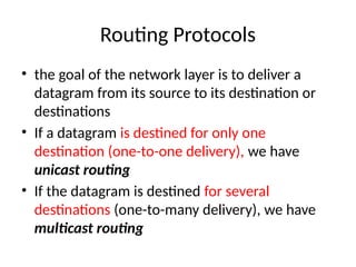
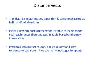
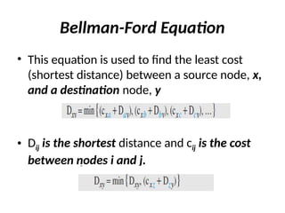
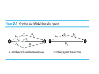
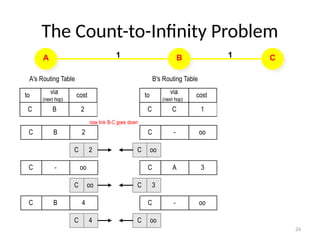
Unicast Routing
Routing Protocols
• the goal of the network layer is to deliver a
datagram from its source to its destination or
destinations
• If a datagram is destined for only one
destination (one-to-one delivery), we have
unicast routing
• If the datagram is destined for several
destinations (one-to-many delivery), we have
multicast routing
Unicast routing – Introduction
• In unicast routing , a packet is routed, hop by
hop, from its source to its destination by the
help of forwarding tables
• the networks in the internet need forwarding
tables.
An Internet as a Graph
• To find the best route, an internet can be
modeled as a graph.
• A graph is a set of nodes and edges (lines) that
connect the nodes.
• each router as a node and each network
between a pair of routers as an edge.
• Each edge is associated with a cost.
Least-Cost Routing
• Best route from the source router to the
destination router is to find the least cost
between the two.
• the source router chooses a route to the
destination router - the total cost for the
route is the least cost among all possible
routes.
Least-Cost Trees
• least-cost tree is a tree with the source router
as the root that spans the whole graph (visits
all other nodes) and in which the path
between the root and any other node is the
shortest.
• shortest-path tree for each node
ROUTING ALGORITHMS
• Distance-Vector Routing (or) Bellman-Ford
Equation
• Link-State Routing
Approaches to Shortest Path Routing
• 1. Link State Routing
– Each node knows the distance to its neighbors
– The distance information (=link state) is broadcast to all nodes in the
network
– Each node calculates the routing tables independently
2. Distance Vector Routing
– Each node knows the distance (=cost) to its directly connected neighbors
– A node sends a list to its neighbors with the current distances to all
nodes
– If all nodes update their distances, the routing tables eventually
converge
Distance Vector
• Each node constructs a one dimensional array (a vector)
containing the “distances” (costs) to all other nodes and
distributes that vector to its immediate neighbors
• Starting assumption is that each node knows the cost of the
link to each of its directly connected neighbors
Distance-vector routing
• the first each node creates is its own least-cost
tree
• The incomplete trees are exchanged between
immediate neighbors to make the trees more and
more complete and to represent the whole
internet.
• A router continuously tells all of its neighbors what
it knows about the whole internet (although the
knowledge can be incomplete)
Distance Vector
Initial distances stored at each node (global view)
Distance Vector
Initial routing table at node A
Distance Vector
Final routing table at node A
Distance Vector
Final distances stored at each node (global view)
Distance Vector
• The distance vector routing algorithm is sometimes called as
Bellman-Ford algorithm
• Every T seconds each router sends its table to its neighbor
each each router then updates its table based on the new
information
• Problems include fast response to good new and slow
response to bad news. Also too many messages to update
Bellman-Ford Equation
• This equation is used to find the least cost
(shortest distance) between a source node, x,
and a destination node, y
• Dij is the shortest distance and cij is the cost
between nodes i and j.
Illustrate the principle of distance vector routing and
apply Bellman-Ford algorithm to find the shortest path
tree for node A (or)
to find routing table for given scenario
23
Characteristics of Distance Vector Routing
• Periodic Updates: Updates to the routing tables are sent at the
end of a certain time period. A typical value is 90 seconds.
• Triggered Updates: If a metric changes on a link, a router
immediately sends out an update without waiting for the end
of the update period.
• Full Routing Table Update: Most distance vector routing
protocol send their neighbors the entire routing table (not only
entries which change).
• Route invalidation timers: Routing table entries are invalid if
they are not refreshed. A typical value is to invalidate an entry
if no update is received after 3-6 update periods.
24
The Count-to-Infinity Problem
A B C
1 1
A's Routing Table B's Routing Table
C
to cost
via
(next hop)
2
B C
to cost
via
(next hop)
1
C
now link B-C goes down
C 2 C oo
C oo
-
C 2
B
C oo C 3
C 3
A
C oo
-
C 4 C oo
C oo
-
C 4
B
25
Count-to-Infinity
• The reason for the count-to-infinity problem is
that each node only has a “next-hop-view”
• For example, in the first step, A did not realize
that its route (with cost 2) to C went through
node B
• How can the Count-to-Infinity problem be
solved?
26
Count-to-Infinity
• The reason for the count-to-infinity problem is that each
node only has a “next-hop-view”
• For example, in the first step, A did not realize that its
route (with cost 2) to C went through node B
• How can the Count-to-Infinity problem be solved?
• Solution 1: Always advertise the entire path in an update
message (Path vectors)
– If routing tables are large, the routing messages require
substantial bandwidth
– BGP uses this solution
27
Count-to-Infinity
• The reason for the count-to-infinity problem is that each
node only has a “next-hop-view”
• For example, in the first step, A did not realize that its route
(with cost 2) to C went through node B
• How can the Count-to-Infinity problem be solved?
• Solution 2: Never advertise the cost to a neighbor if this
neighbor is the next hop on the current path (Split Horizon)
– Example: A would not send the first routing update to B, since B is the next hop
on A’s current route to C
– Split Horizon does not solve count-to-infinity in all cases!
28
Link State Routing
Link State Routing
Strategy: Send to all nodes (not just neighbors) information
about directly connected links (not entire routing table).
• Link State Packet (LSP)
– id of the node that created the LSP
– cost of link to each directly connected neighbor
– sequence number (SEQNO)
– time-to-live (TTL) for this packet
• Reliable Flooding
– store most recent LSP from each node
– forward LSP to all nodes but one that sent it
– generate new LSP periodically; increment SEQNO
– start SEQNO at 0 when reboot
– decrement TTL of each stored LSP; discard when TTL=0
30
Link State Routing
• In link state routing, each node has a complete map of
the topology
• If a node fails, each
node can calculate
the new route
• Difficulty:All nodes need to
have a consistent view of the
network
A B C
D E F
A B C
D E F
A B C
D E F
A B C
D E F
A B C
D E F
A B C
D E F
A B C
D E F
Link State Routing
• Each node must
– discover its neighbors
– measure the delay (=cost) to its neighbors
– broadcast a packet with this information to all other nodes
– compute the shortest paths to every other router
• The broadcast can be accomplished by flooding
• The shortest paths can be computer with Dijkstra’s
algorithm
32
Link State Routing: Basic princples
1. Each router establishes a relationship (“adjacency”)
with its neighbors
2.Each router generates link state advertisements (LSAs)
which are distributed to all routers
LSA = (link id, state of the link, cost, neighbors of the link)
3. Each router maintains a database of all received LSAs
(topological database or link state database), which
describes the network has a graph with weighted edges
4. Each router uses its link state database to run a
shortest path algorithm (Dijikstra’s algorithm) to
produce the shortest path to each network
33
Link State Routing: Properties
• Each node requires complete topology
information
• Link state information must be flooded to all
nodes
• Guaranteed to converge
Link State
Reliable Flooding
Flooding of link-state packets. (a) LSP arrives at node X; (b) X floods LSP to A
and C; (c) A and C flood LSP to B (but not X); (d) flooding is complete
35
Dijkstra’s Shortest Path Algorithm for a Graph
Input: Graph (N,E) with
N the set of nodes and E  N × N the set of edges
dvw link cost (dvw = infinity if (v,w)  E, dvv = 0)
s source node.
Output: Dn cost of the least-cost path from node s to node n
M = {s};
for each n  M
Dn = dsn;
while (M  all nodes) do
Find w  M for which Dw = min{Dj ; j  M};
Add w to M;
for each n  M
Dn = minw [ Dn, Dw + dwn ];
Update route;
enddo
Shortest Path Routing
39
Example Network
1
2 3
4 5
6
5
2
1
1
1
2
2
3
3
5

Computer Network - Unicast Routing Distance vector Link state vector

  • 1.
  • 2.
    Routing Protocols • thegoal of the network layer is to deliver a datagram from its source to its destination or destinations • If a datagram is destined for only one destination (one-to-one delivery), we have unicast routing • If the datagram is destined for several destinations (one-to-many delivery), we have multicast routing
  • 3.
    Unicast routing –Introduction • In unicast routing , a packet is routed, hop by hop, from its source to its destination by the help of forwarding tables • the networks in the internet need forwarding tables.
  • 4.
    An Internet asa Graph • To find the best route, an internet can be modeled as a graph. • A graph is a set of nodes and edges (lines) that connect the nodes. • each router as a node and each network between a pair of routers as an edge. • Each edge is associated with a cost.
  • 5.
    Least-Cost Routing • Bestroute from the source router to the destination router is to find the least cost between the two. • the source router chooses a route to the destination router - the total cost for the route is the least cost among all possible routes.
  • 7.
    Least-Cost Trees • least-costtree is a tree with the source router as the root that spans the whole graph (visits all other nodes) and in which the path between the root and any other node is the shortest. • shortest-path tree for each node
  • 9.
    ROUTING ALGORITHMS • Distance-VectorRouting (or) Bellman-Ford Equation • Link-State Routing
  • 10.
    Approaches to ShortestPath Routing • 1. Link State Routing – Each node knows the distance to its neighbors – The distance information (=link state) is broadcast to all nodes in the network – Each node calculates the routing tables independently 2. Distance Vector Routing – Each node knows the distance (=cost) to its directly connected neighbors – A node sends a list to its neighbors with the current distances to all nodes – If all nodes update their distances, the routing tables eventually converge
  • 11.
    Distance Vector • Eachnode constructs a one dimensional array (a vector) containing the “distances” (costs) to all other nodes and distributes that vector to its immediate neighbors • Starting assumption is that each node knows the cost of the link to each of its directly connected neighbors
  • 12.
    Distance-vector routing • thefirst each node creates is its own least-cost tree • The incomplete trees are exchanged between immediate neighbors to make the trees more and more complete and to represent the whole internet. • A router continuously tells all of its neighbors what it knows about the whole internet (although the knowledge can be incomplete)
  • 13.
    Distance Vector Initial distancesstored at each node (global view)
  • 14.
  • 15.
  • 16.
    Distance Vector Final distancesstored at each node (global view)
  • 17.
    Distance Vector • Thedistance vector routing algorithm is sometimes called as Bellman-Ford algorithm • Every T seconds each router sends its table to its neighbor each each router then updates its table based on the new information • Problems include fast response to good new and slow response to bad news. Also too many messages to update
  • 18.
    Bellman-Ford Equation • Thisequation is used to find the least cost (shortest distance) between a source node, x, and a destination node, y • Dij is the shortest distance and cij is the cost between nodes i and j.
  • 20.
    Illustrate the principleof distance vector routing and apply Bellman-Ford algorithm to find the shortest path tree for node A (or) to find routing table for given scenario
  • 23.
    23 Characteristics of DistanceVector Routing • Periodic Updates: Updates to the routing tables are sent at the end of a certain time period. A typical value is 90 seconds. • Triggered Updates: If a metric changes on a link, a router immediately sends out an update without waiting for the end of the update period. • Full Routing Table Update: Most distance vector routing protocol send their neighbors the entire routing table (not only entries which change). • Route invalidation timers: Routing table entries are invalid if they are not refreshed. A typical value is to invalidate an entry if no update is received after 3-6 update periods.
  • 24.
    24 The Count-to-Infinity Problem AB C 1 1 A's Routing Table B's Routing Table C to cost via (next hop) 2 B C to cost via (next hop) 1 C now link B-C goes down C 2 C oo C oo - C 2 B C oo C 3 C 3 A C oo - C 4 C oo C oo - C 4 B
  • 25.
    25 Count-to-Infinity • The reasonfor the count-to-infinity problem is that each node only has a “next-hop-view” • For example, in the first step, A did not realize that its route (with cost 2) to C went through node B • How can the Count-to-Infinity problem be solved?
  • 26.
    26 Count-to-Infinity • The reasonfor the count-to-infinity problem is that each node only has a “next-hop-view” • For example, in the first step, A did not realize that its route (with cost 2) to C went through node B • How can the Count-to-Infinity problem be solved? • Solution 1: Always advertise the entire path in an update message (Path vectors) – If routing tables are large, the routing messages require substantial bandwidth – BGP uses this solution
  • 27.
    27 Count-to-Infinity • The reasonfor the count-to-infinity problem is that each node only has a “next-hop-view” • For example, in the first step, A did not realize that its route (with cost 2) to C went through node B • How can the Count-to-Infinity problem be solved? • Solution 2: Never advertise the cost to a neighbor if this neighbor is the next hop on the current path (Split Horizon) – Example: A would not send the first routing update to B, since B is the next hop on A’s current route to C – Split Horizon does not solve count-to-infinity in all cases!
  • 28.
  • 29.
    Link State Routing Strategy:Send to all nodes (not just neighbors) information about directly connected links (not entire routing table). • Link State Packet (LSP) – id of the node that created the LSP – cost of link to each directly connected neighbor – sequence number (SEQNO) – time-to-live (TTL) for this packet • Reliable Flooding – store most recent LSP from each node – forward LSP to all nodes but one that sent it – generate new LSP periodically; increment SEQNO – start SEQNO at 0 when reboot – decrement TTL of each stored LSP; discard when TTL=0
  • 30.
    30 Link State Routing •In link state routing, each node has a complete map of the topology • If a node fails, each node can calculate the new route • Difficulty:All nodes need to have a consistent view of the network A B C D E F A B C D E F A B C D E F A B C D E F A B C D E F A B C D E F A B C D E F
  • 31.
    Link State Routing •Each node must – discover its neighbors – measure the delay (=cost) to its neighbors – broadcast a packet with this information to all other nodes – compute the shortest paths to every other router • The broadcast can be accomplished by flooding • The shortest paths can be computer with Dijkstra’s algorithm
  • 32.
    32 Link State Routing:Basic princples 1. Each router establishes a relationship (“adjacency”) with its neighbors 2.Each router generates link state advertisements (LSAs) which are distributed to all routers LSA = (link id, state of the link, cost, neighbors of the link) 3. Each router maintains a database of all received LSAs (topological database or link state database), which describes the network has a graph with weighted edges 4. Each router uses its link state database to run a shortest path algorithm (Dijikstra’s algorithm) to produce the shortest path to each network
  • 33.
    33 Link State Routing:Properties • Each node requires complete topology information • Link state information must be flooded to all nodes • Guaranteed to converge
  • 34.
    Link State Reliable Flooding Floodingof link-state packets. (a) LSP arrives at node X; (b) X floods LSP to A and C; (c) A and C flood LSP to B (but not X); (d) flooding is complete
  • 35.
    35 Dijkstra’s Shortest PathAlgorithm for a Graph Input: Graph (N,E) with N the set of nodes and E  N × N the set of edges dvw link cost (dvw = infinity if (v,w)  E, dvv = 0) s source node. Output: Dn cost of the least-cost path from node s to node n M = {s}; for each n  M Dn = dsn; while (M  all nodes) do Find w  M for which Dw = min{Dj ; j  M}; Add w to M; for each n  M Dn = minw [ Dn, Dw + dwn ]; Update route; enddo
  • 38.
  • 39.
    39 Example Network 1 2 3 45 6 5 2 1 1 1 2 2 3 3 5