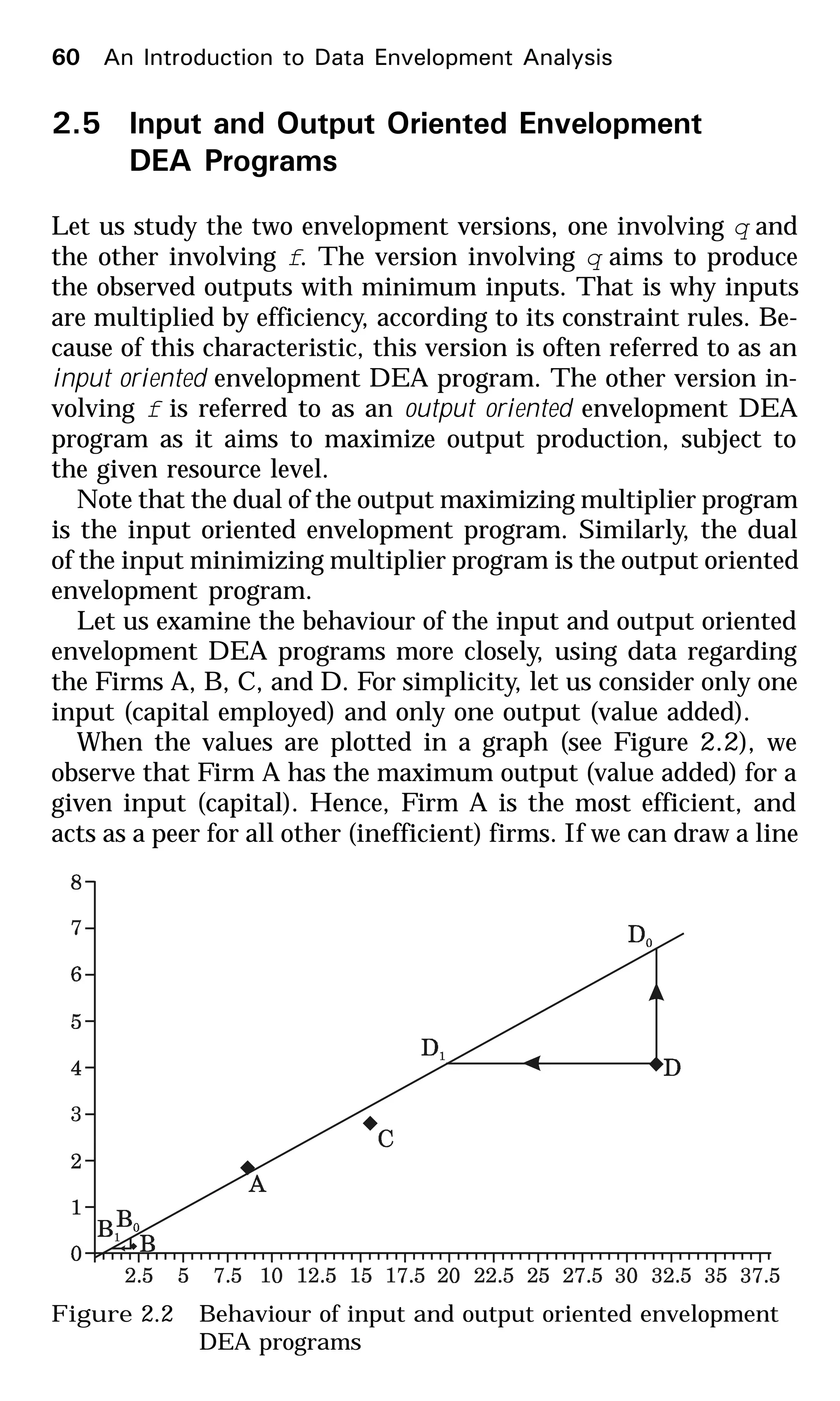
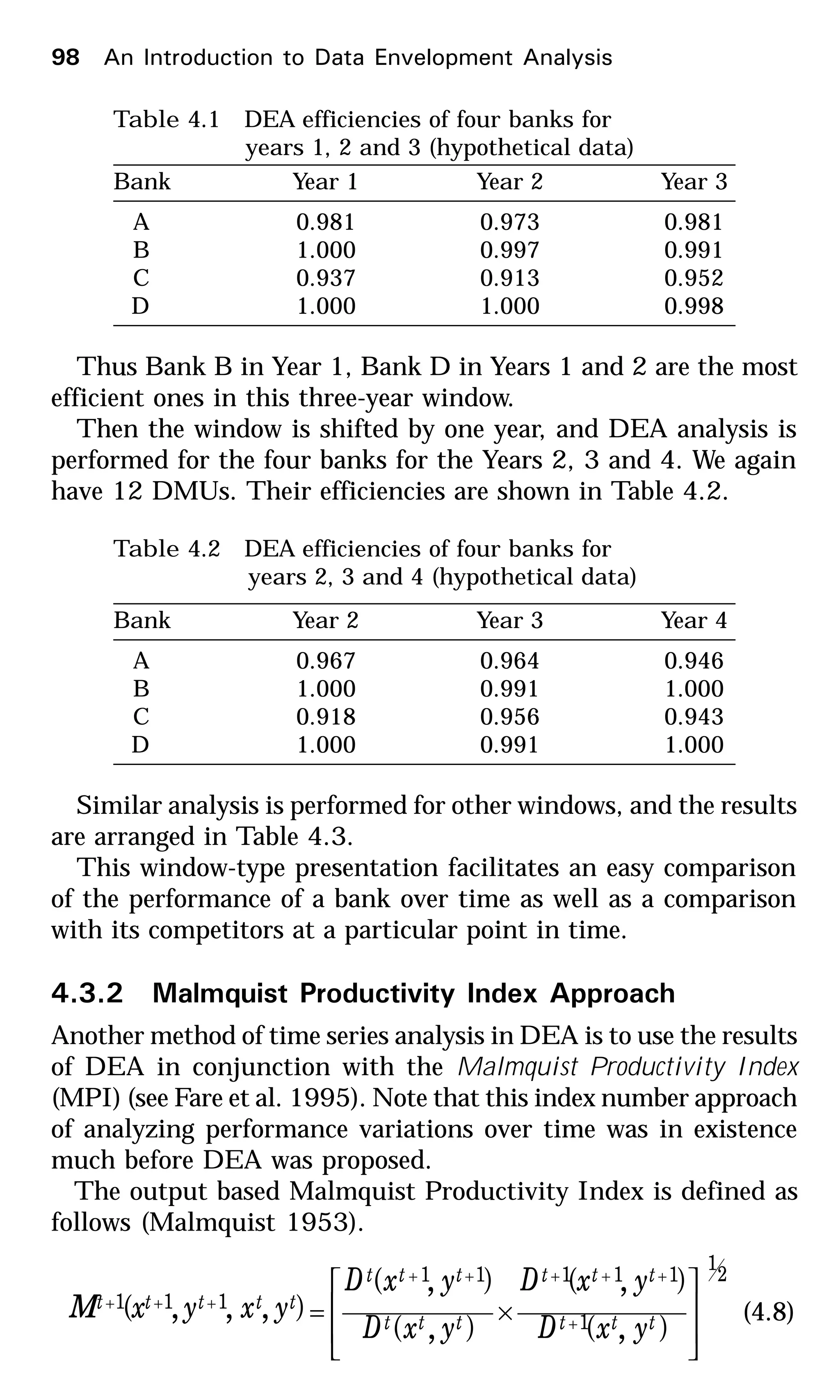
This document provides an introduction to data envelopment analysis (DEA). It begins with basic concepts of efficiency measurement using DEA, including graphical frontier analysis. It then discusses the mathematical programming aspects of DEA, including both primal and dual formulations. It also covers extensions to DEA such as variable returns to scale and window analysis. The document concludes with a discussion of DEA software, applications of DEA in various fields, and strengths and limitations of the approach.


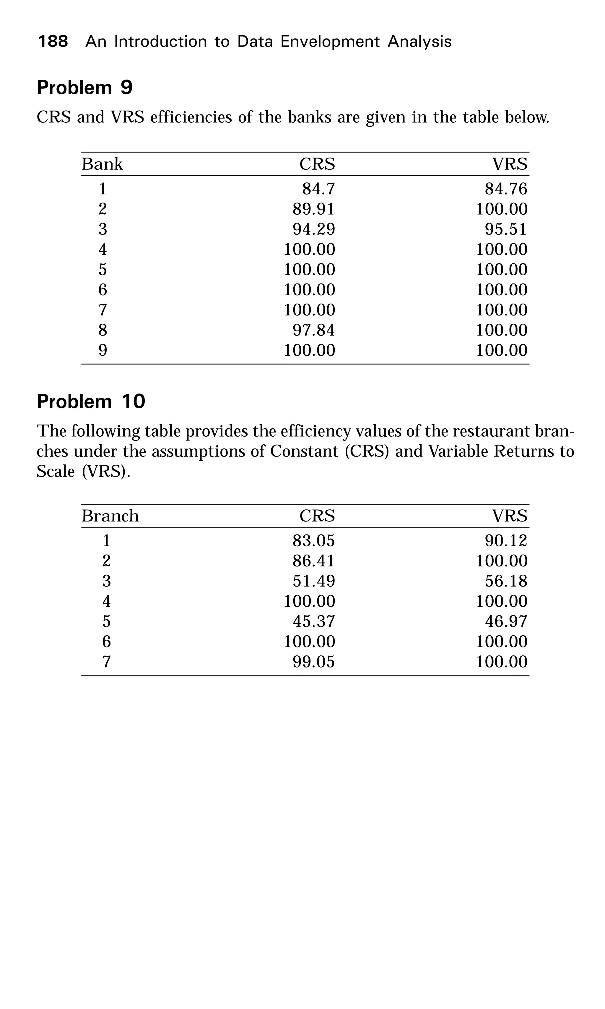
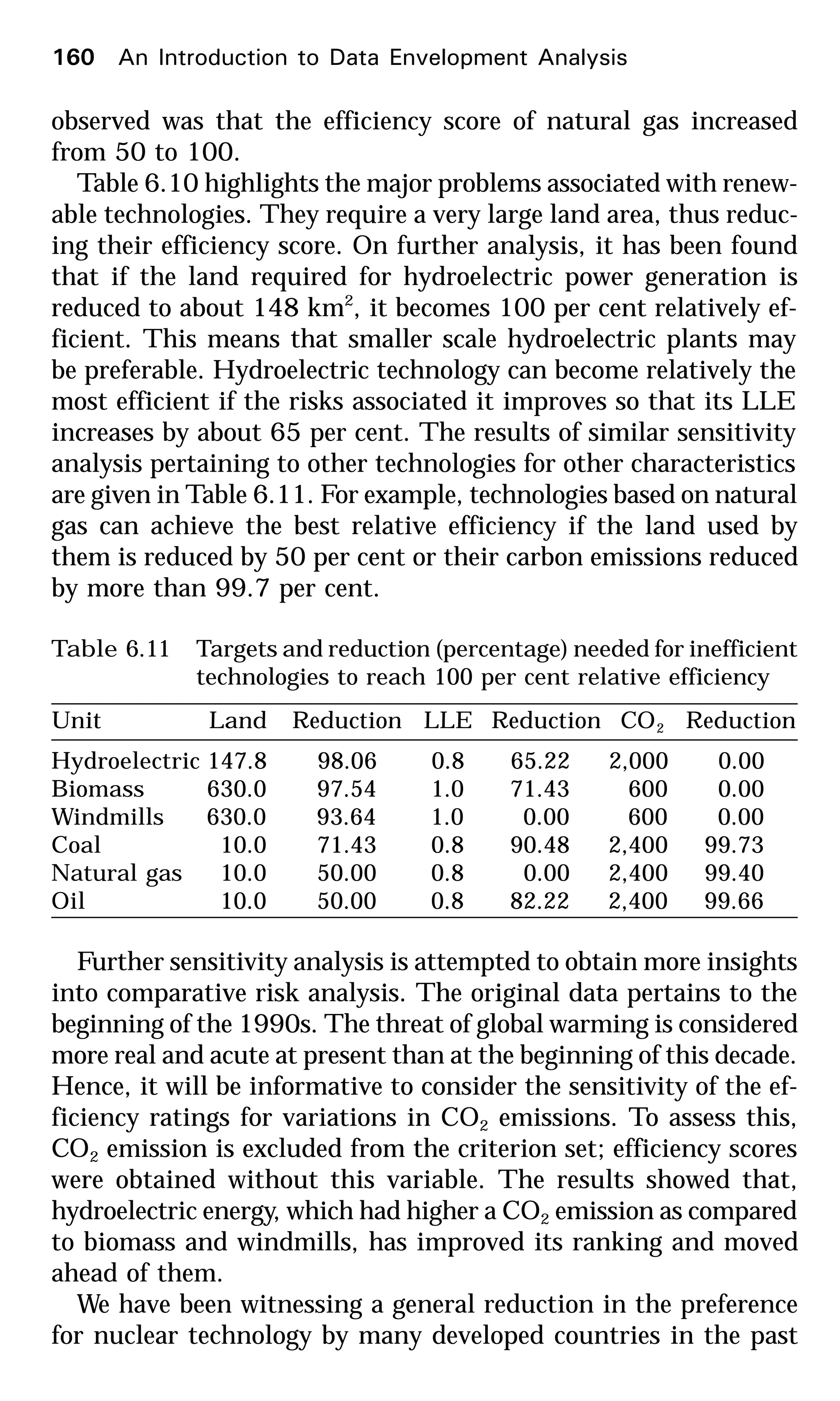
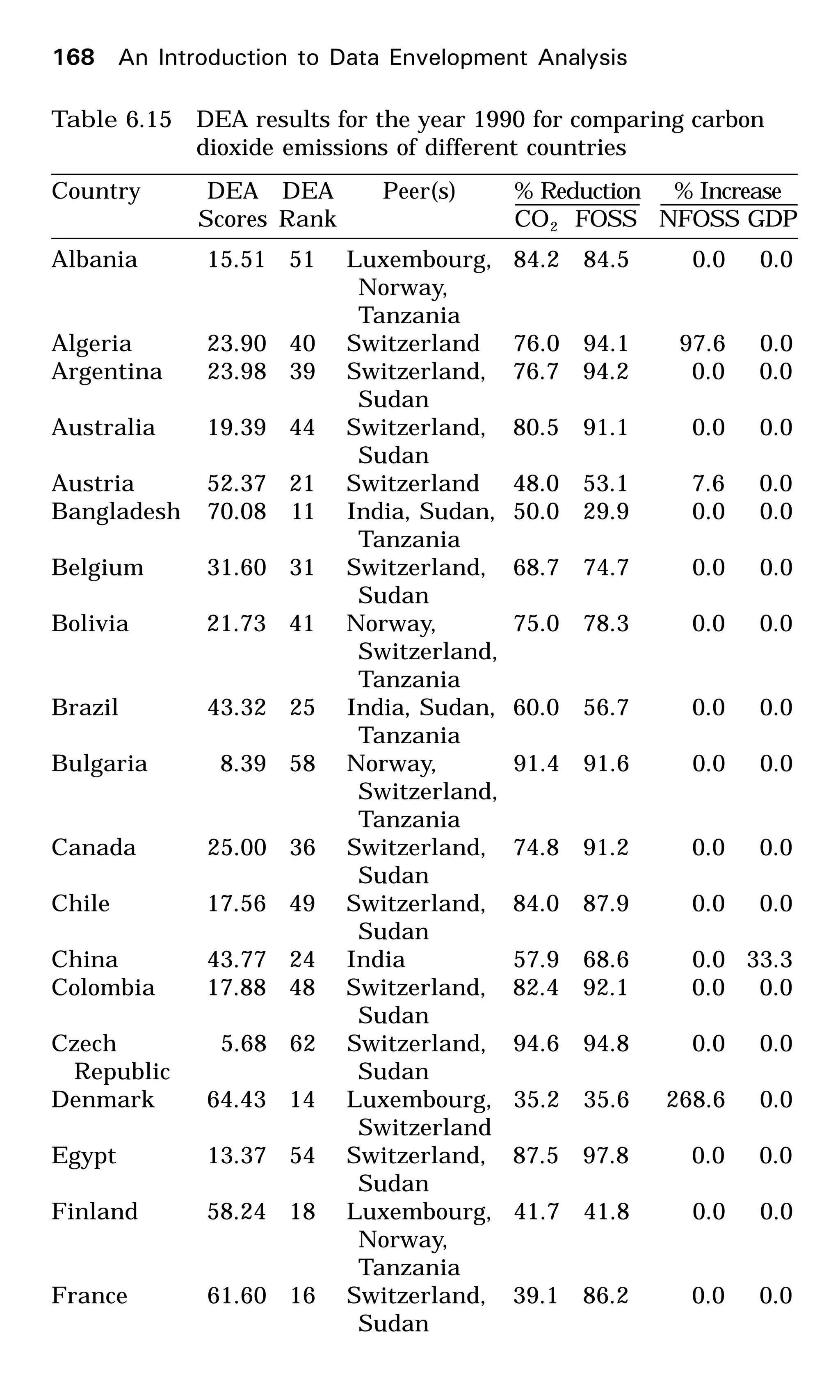
![(d) M operates at its MPSS.
(e) Firm P is 100 per cent scale efficient.
( f ) If one introduces the constraint ål ³ 1 to the CCR
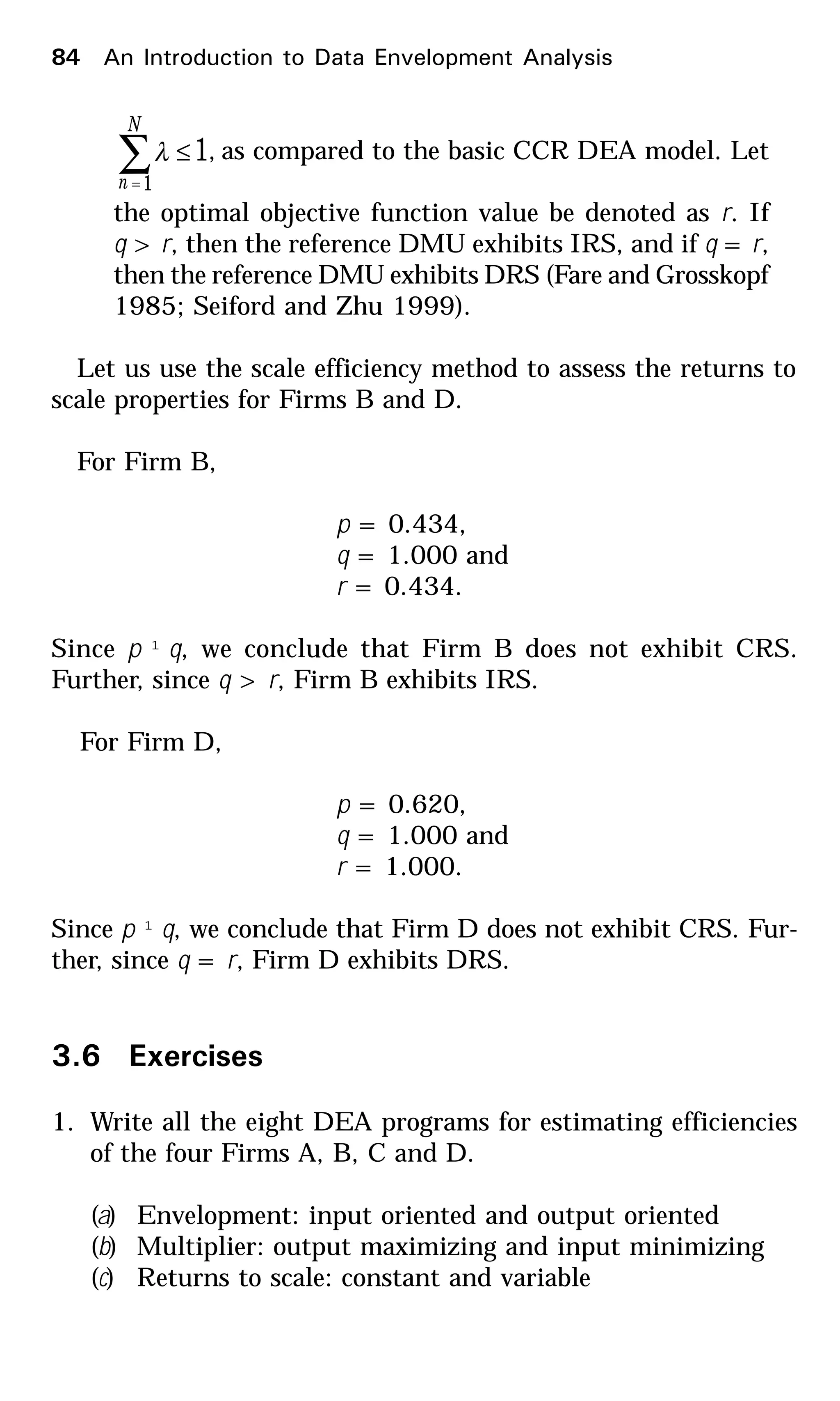
envelopment model, Firm M will be considered effi-
cient.
(g) Write the ratios for the CRS, VRS and scale efficiencies
of Firm A.
The following questions have been included as practice prob-
lems for demonstrating the variety of applications of DEA.
Several applications of DEA have been described in Chap-
ter 6, each for of which the data and the DEA results have
been presented. Students should consider them also as practice
problems. In addition, several data sets for practicing DEA
are available on the Internet. See Chapter 5 for more details.
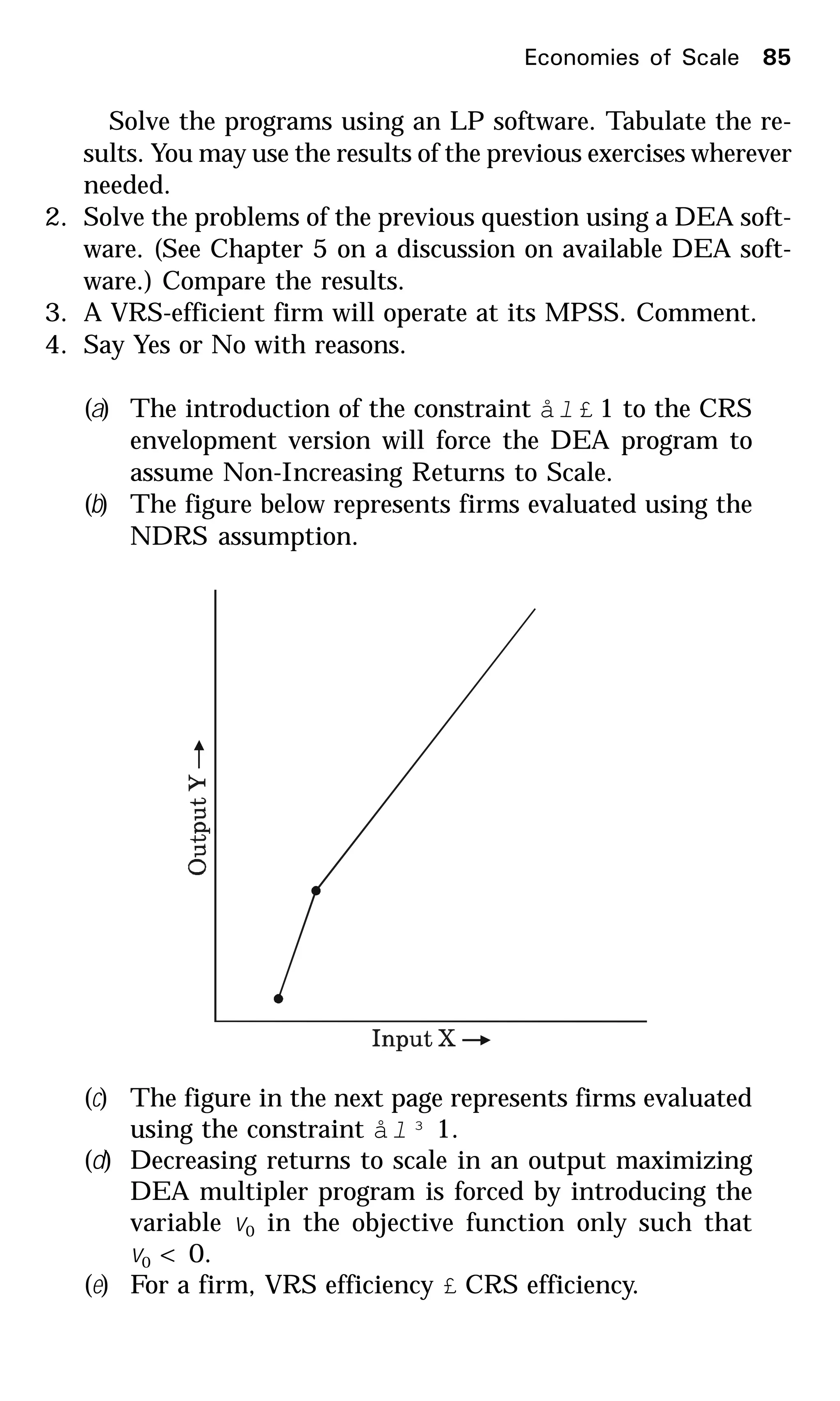
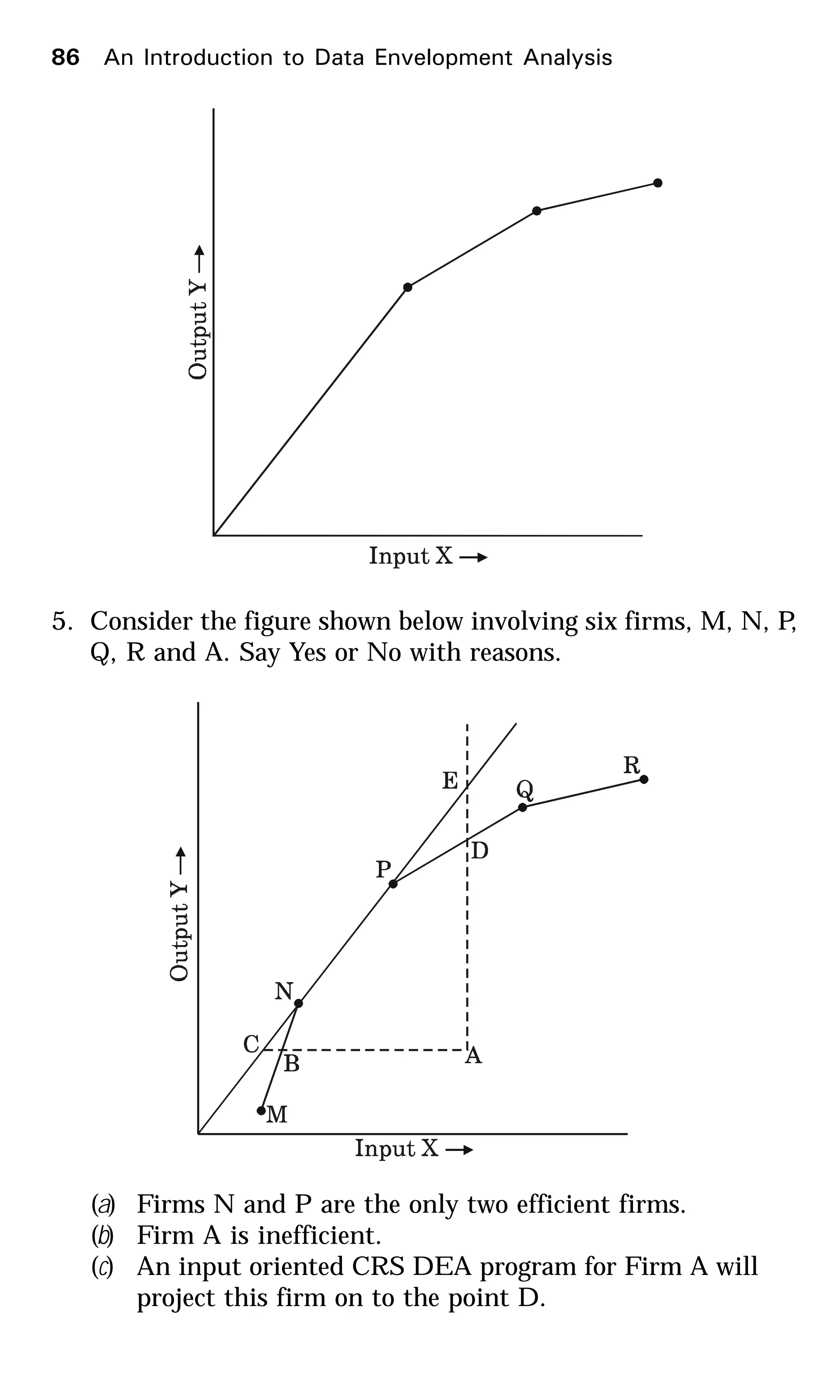
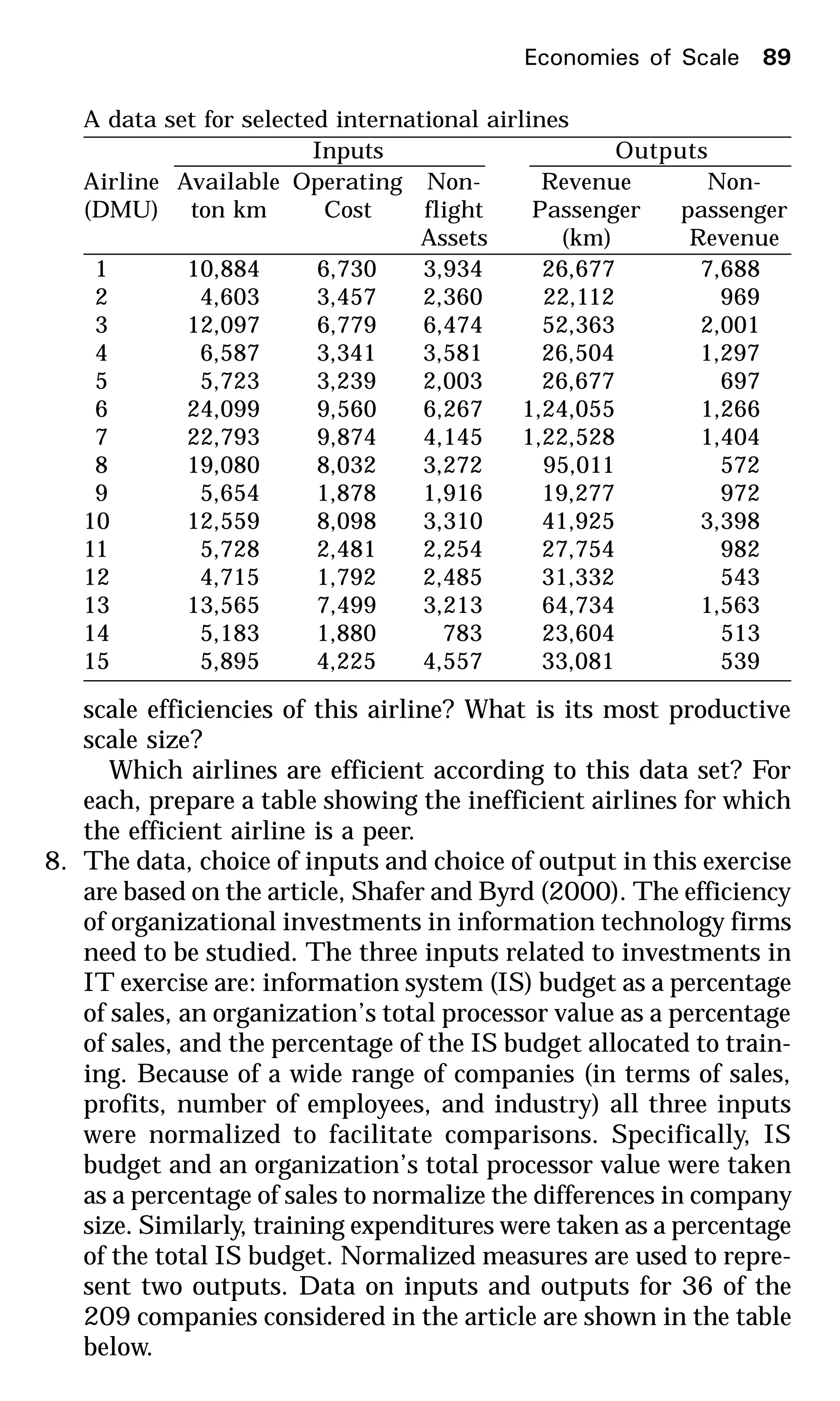
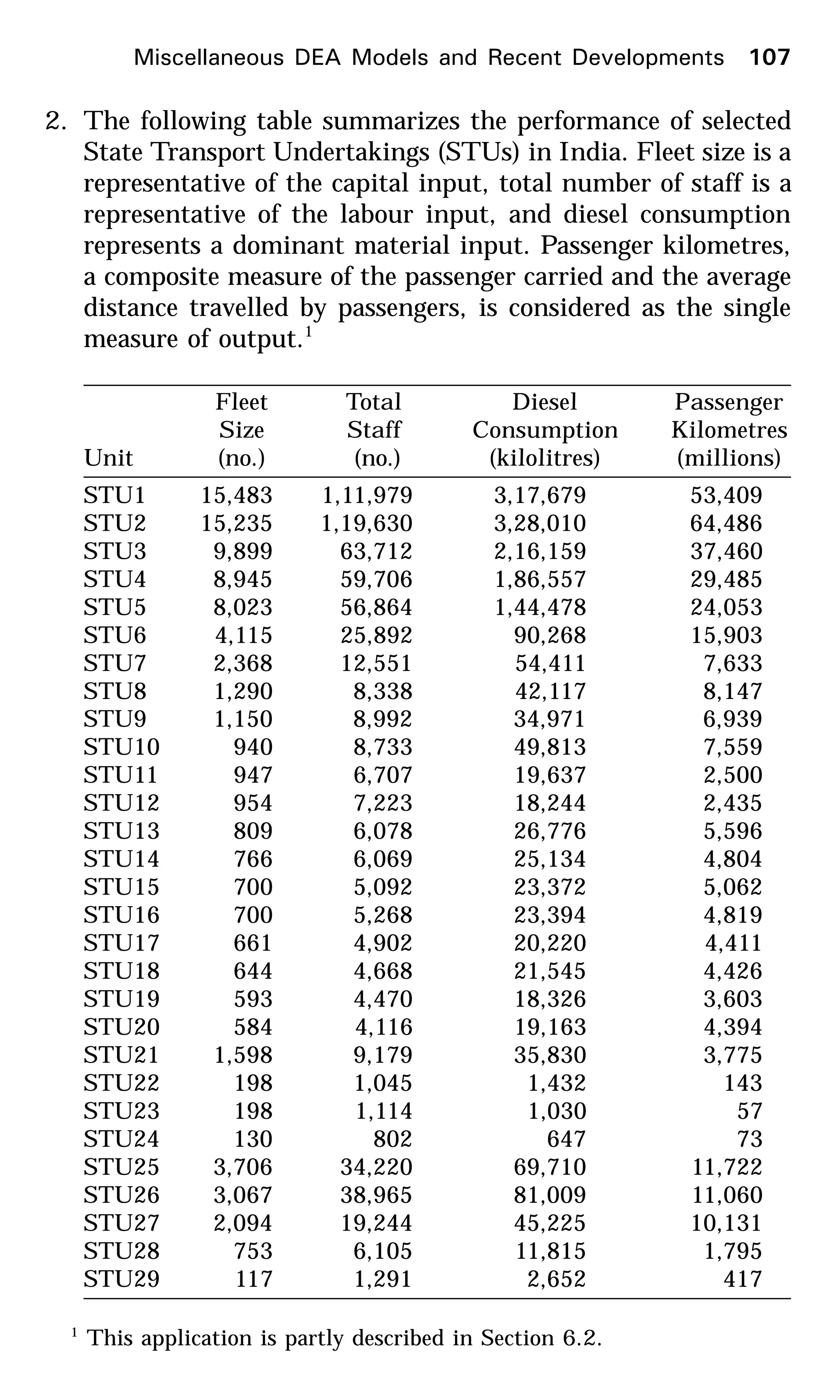
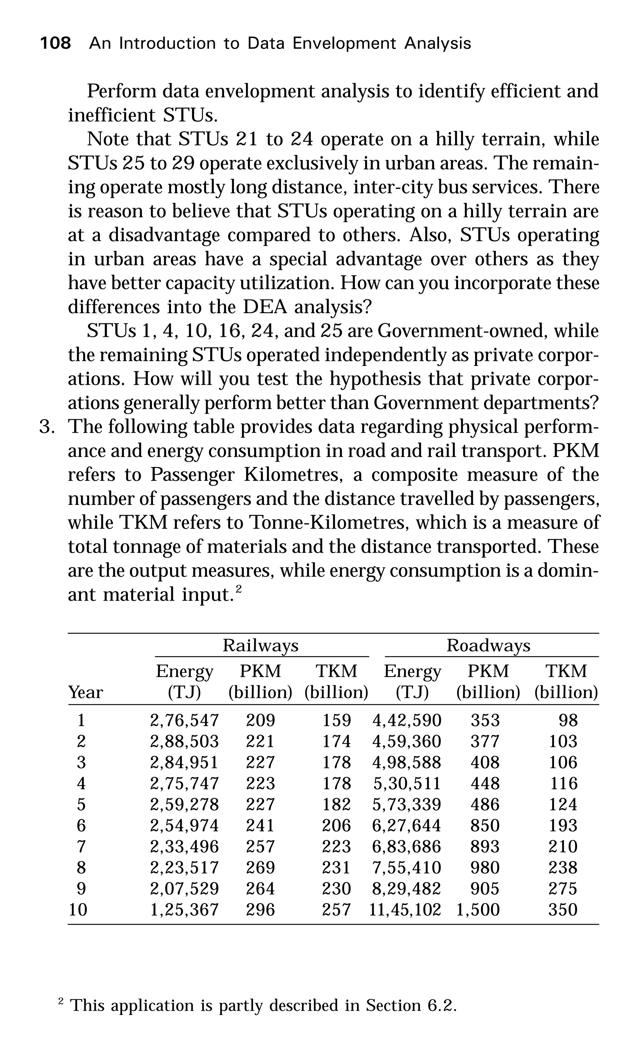
6. The data, choice of inputs and choice of output in this exercise
are based on the article, Sueyoshi and Goto (2001). The fol-
lowing data represents, for the year 1993, three inputs (the
amount of total fossil fuel generation capacity in Mega Watts
(MW); the amount of total fuel consumption in 109
kilocalories
(kcal); and the number of total employees in fossil fuel plants)
and one output (the amount of total generation in Giga Watt-
hour [GWh]) pertaining to electric power generation companies
in Japan.
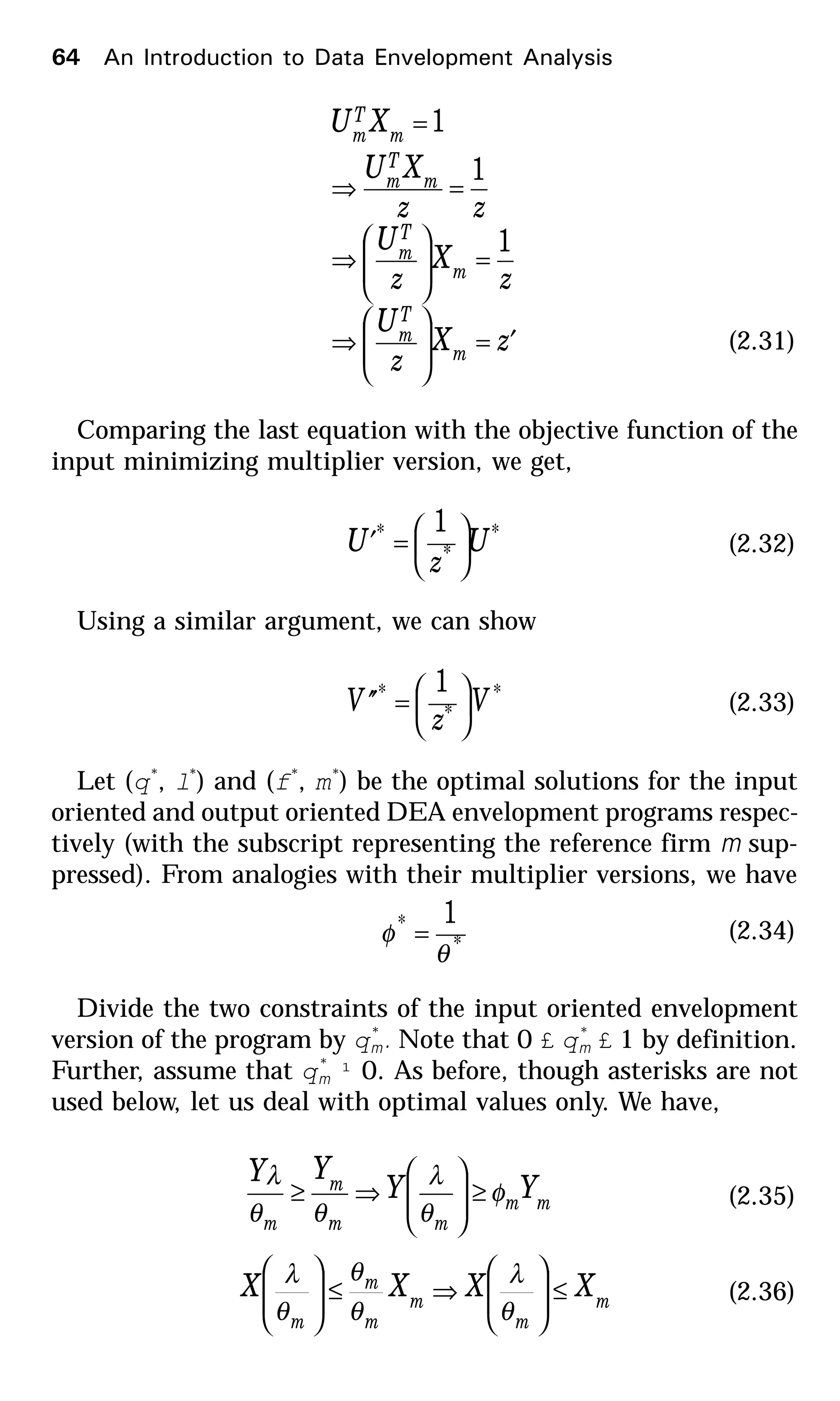
Write all the eight DEA programs (Envelopment: input
oriented and output oriented, Multiplier: output maximizing
and input minimizing, and Returns to scale: constant and
variable) for estimating the efficiency of the power generation
company located in Hokkaido.
Solve the programs using an LP software. Tabulate the re-
sults. Is the Hokkaido power generation company efficient?
If not, which power generation companies would you recom-
mend the Hokkaido company consider emulating to improve
the efficiency of its operation? What are the CRS, VRS and
scale efficiencies of this company? What is its most productive
scale size?
Which are the efficient power generation companies in this
data set? For each of them, prepare a table showing the ineffi-
cient companies for whom the efficient company is a peer.
Economies of Scale 87](https://image.slidesharecdn.com/anintroductiontodea-180619020626/75/An-introduction-to-dea-88-2048.jpg)
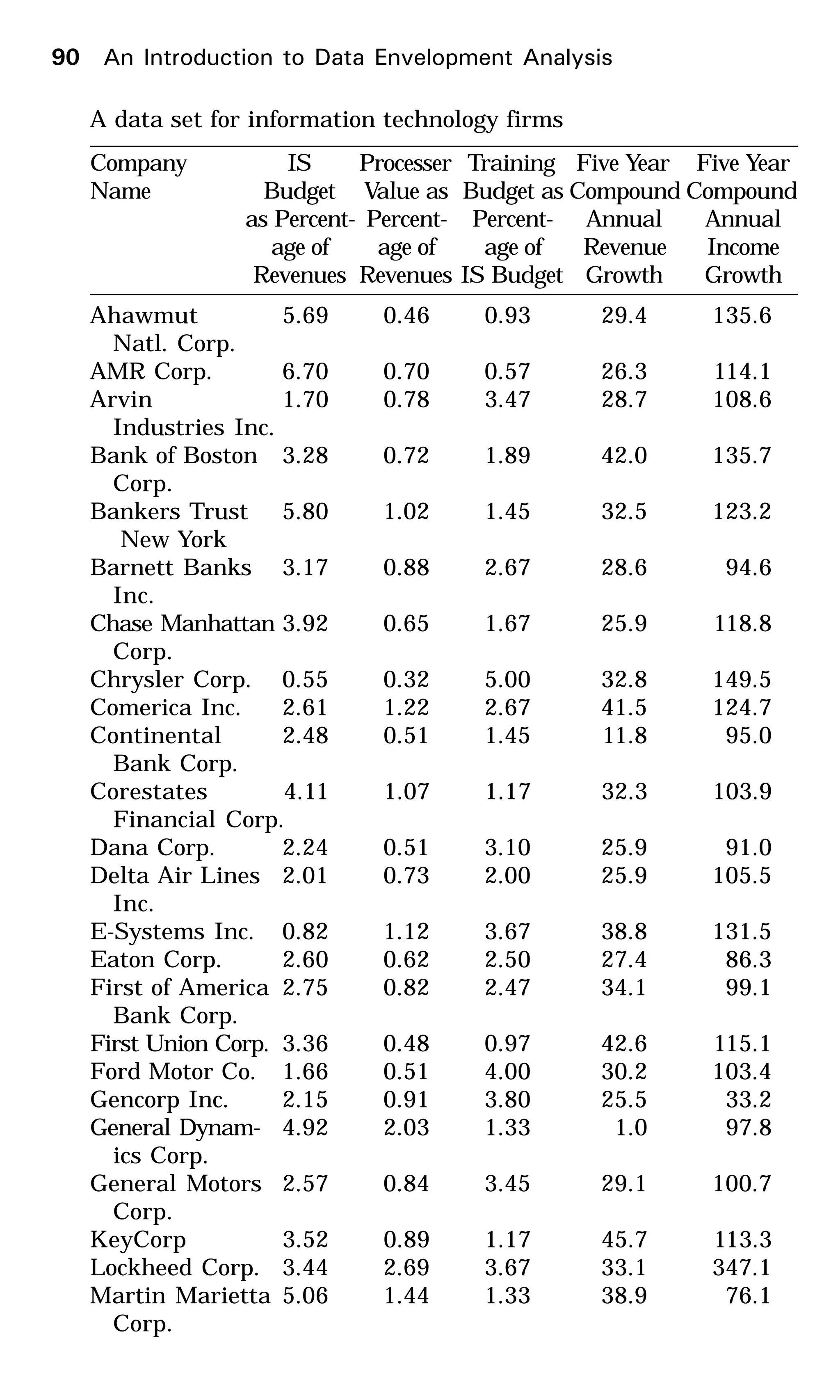

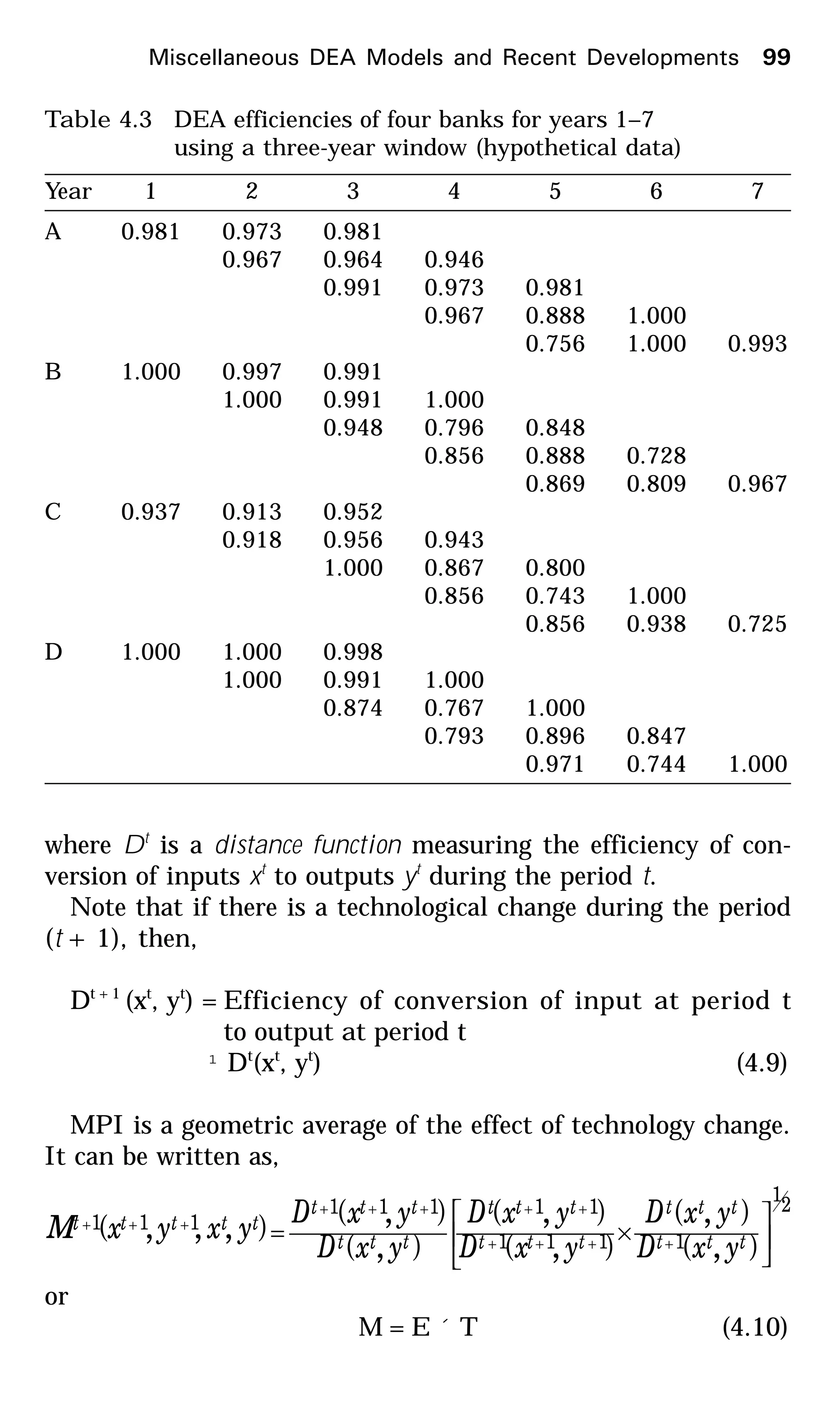
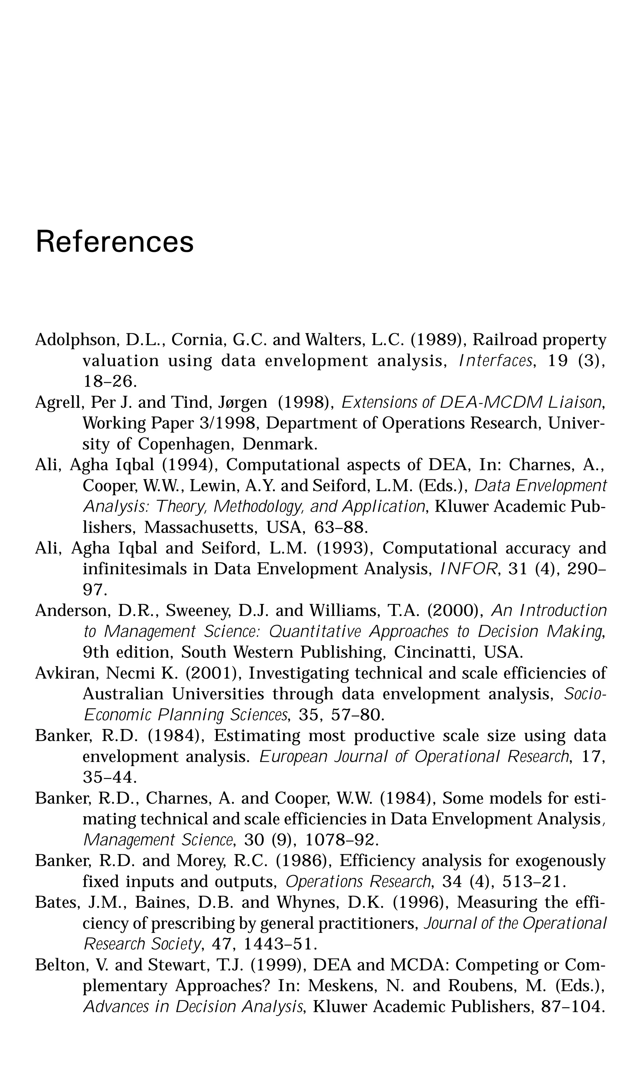
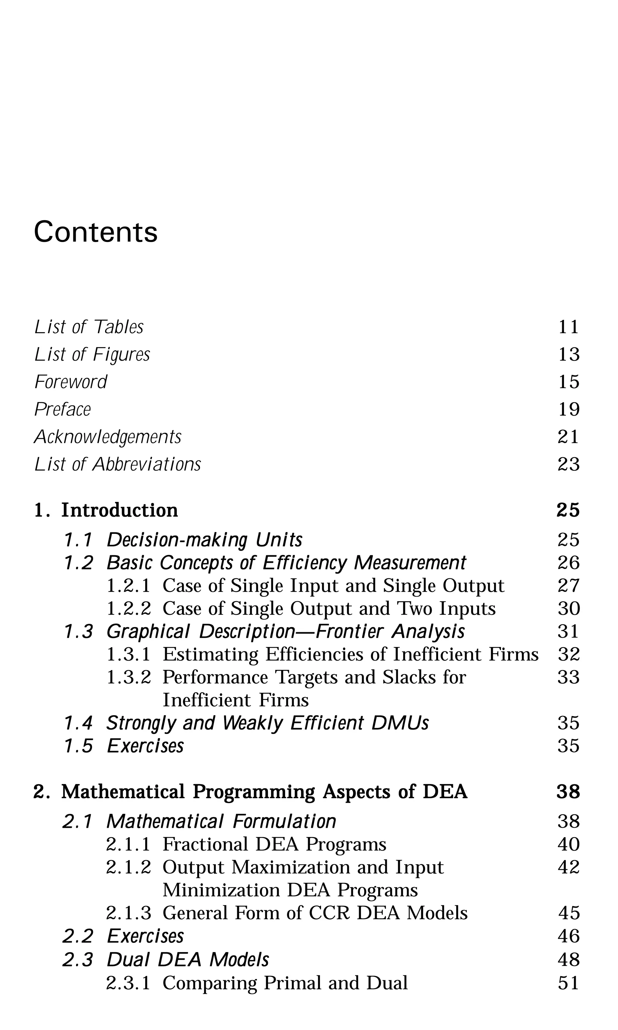
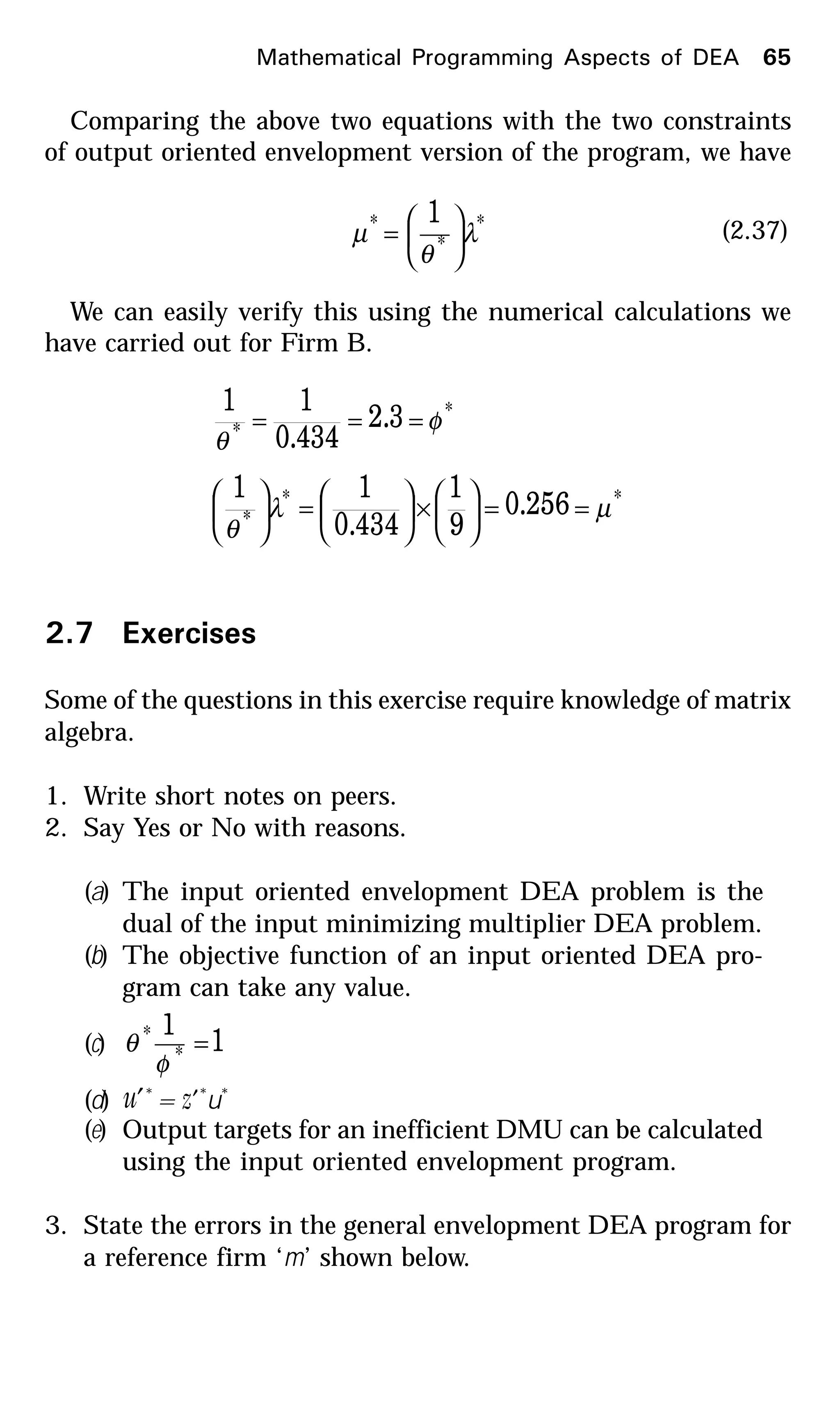
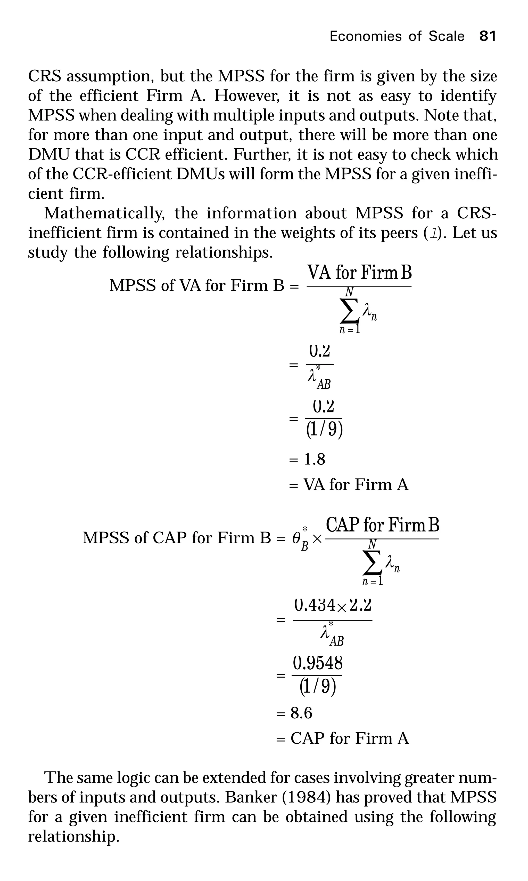
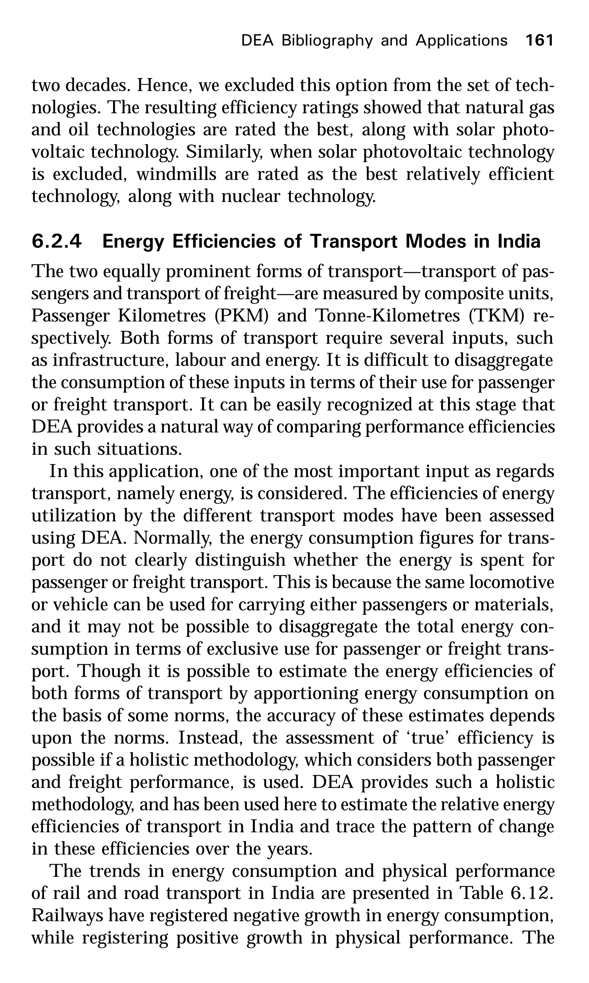
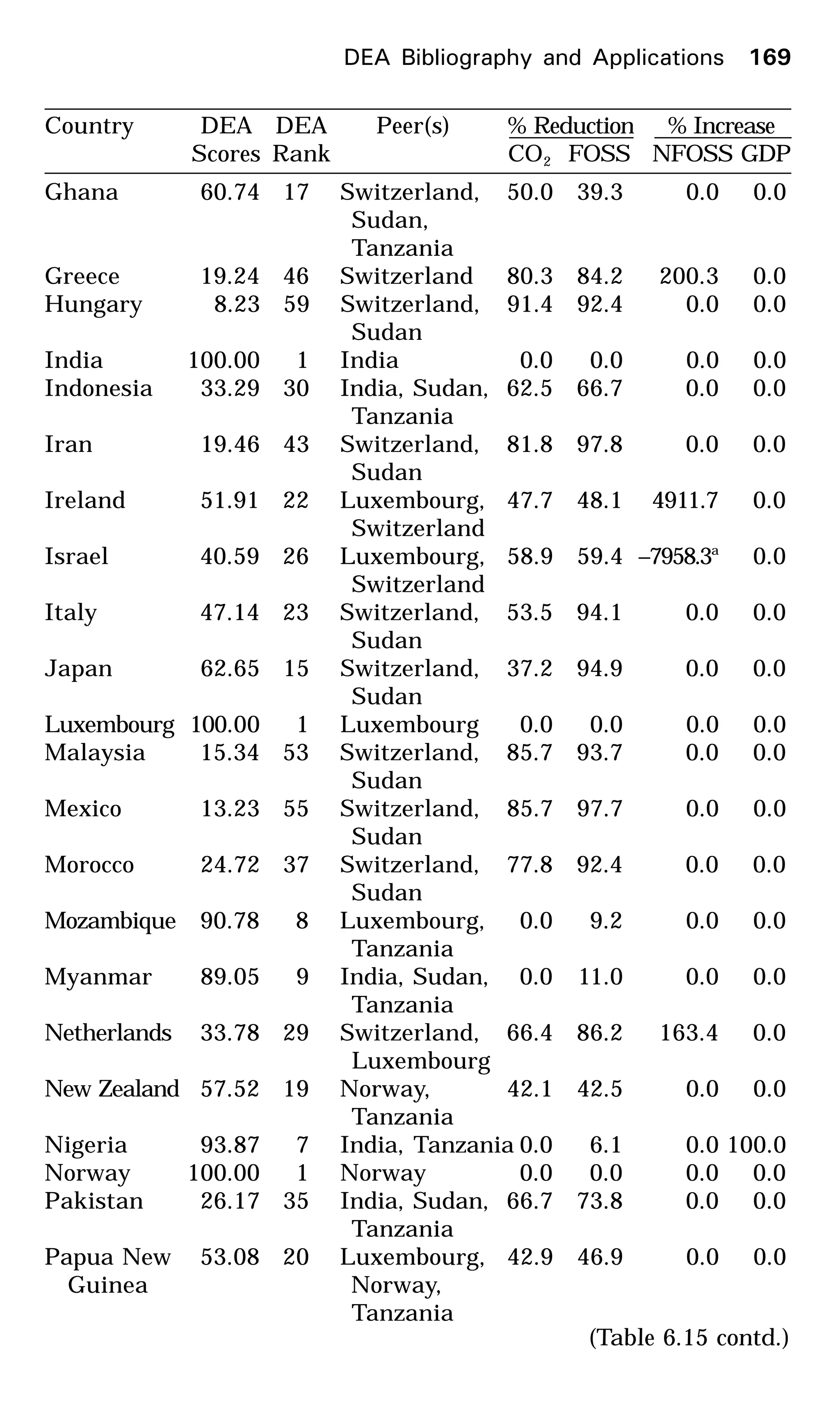
![Similarly,
( )
OE
OF
yxD ttt =,
Hence,
( )
( )
( )
( )OEOF
OAOB
yxD
yxD
E
ttt
ttt
/
/
,
,
changeefficiencyTechnical
111
=
=
=
+++
(4.11)
If E > 1, then there is an increase in the technical efficiency of
converting inputs to outputs.
What does ( )[ ]ttt yxD , ( )[ ]ttt yxD ,1+
in Equation 4.10 mean?
Because of a technical change, the same input xt
can produce a
higher output when used during the period (t+1). Input xt
can
produce only OE as its best ouput in time t, but can produce a
higher output OC in time (t+1). Hence, the ratio (OC/OE)
represents a measure of technology change. If this ratio is greater
than unity, then there is proof of technological improvement.
( )
( )
OC
OFyxD
OE
OF
yxD
ttt
ttt
=
=
+
,
,
1
HHence,
( )
( ) OE
OC
yxD
yxD
ttt
ttt
=+
,
,
1
For technological progress, this ratio should be greater than
unity. Similarly,
( )
( )
1
,
,
111
11
>=
+++
++
OD
OA
yxD
yxD
ttt
ttt
for technological progress.
Miscellaneous DEA Models and Recent Developments 101](https://image.slidesharecdn.com/anintroductiontodea-180619020626/75/An-introduction-to-dea-102-2048.jpg)

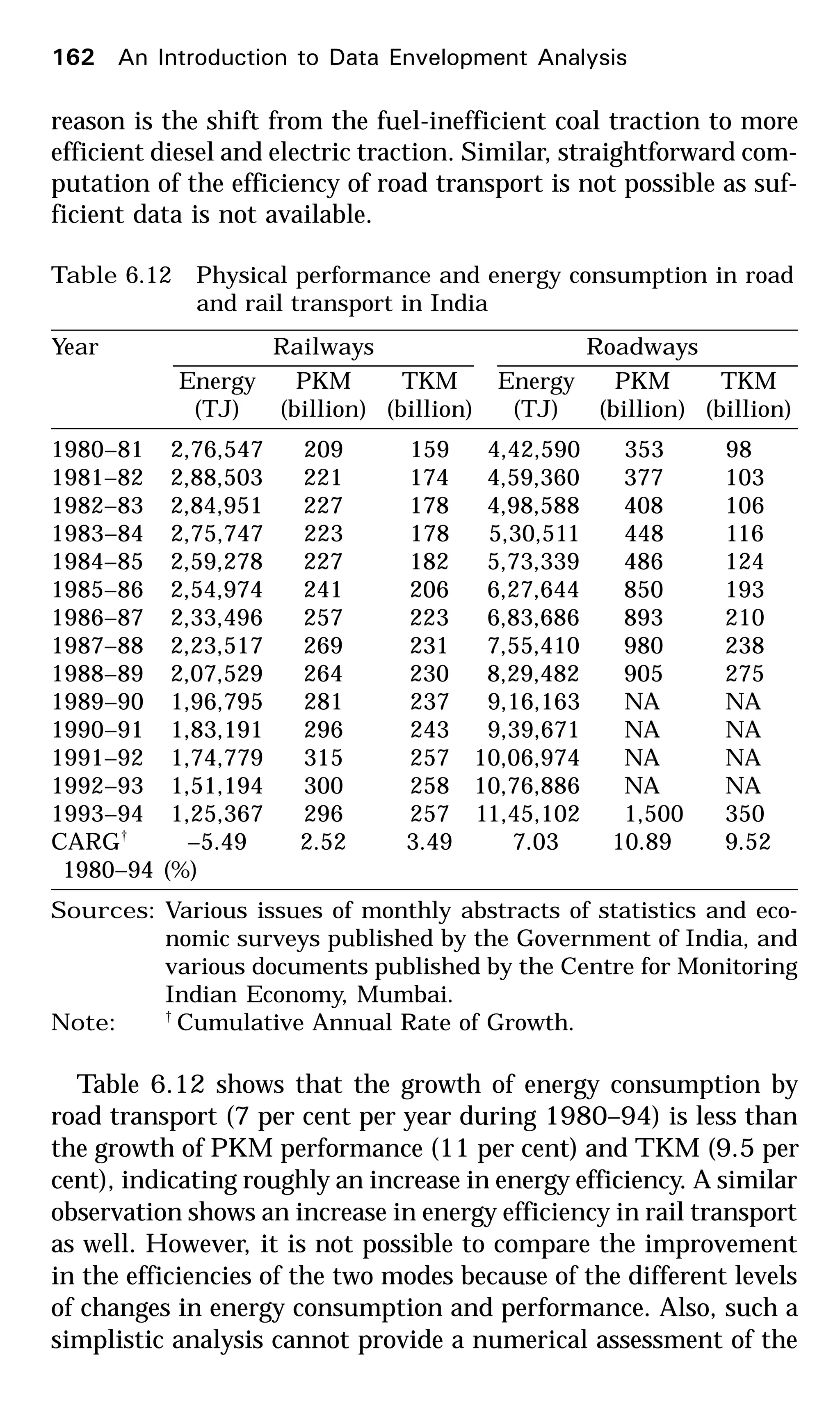
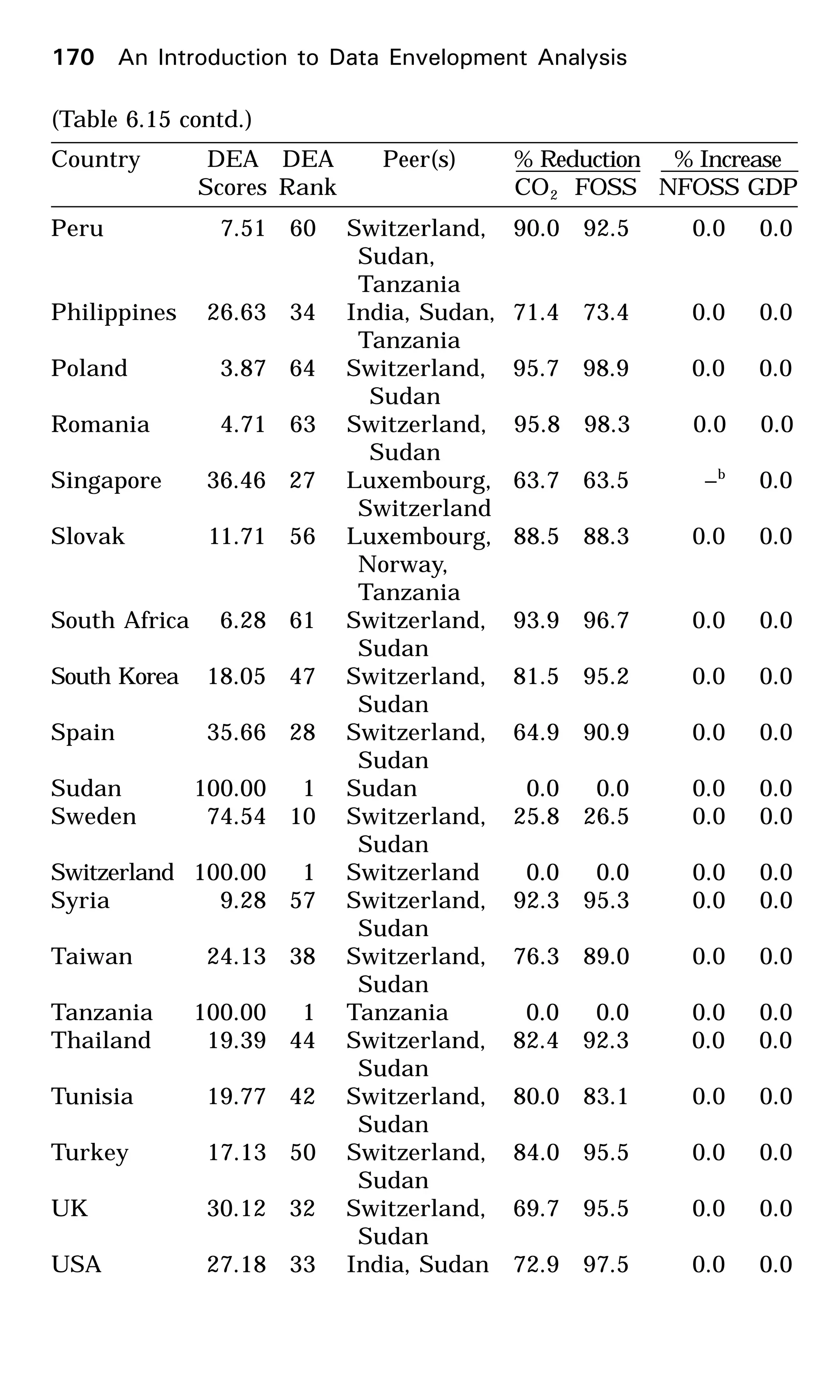
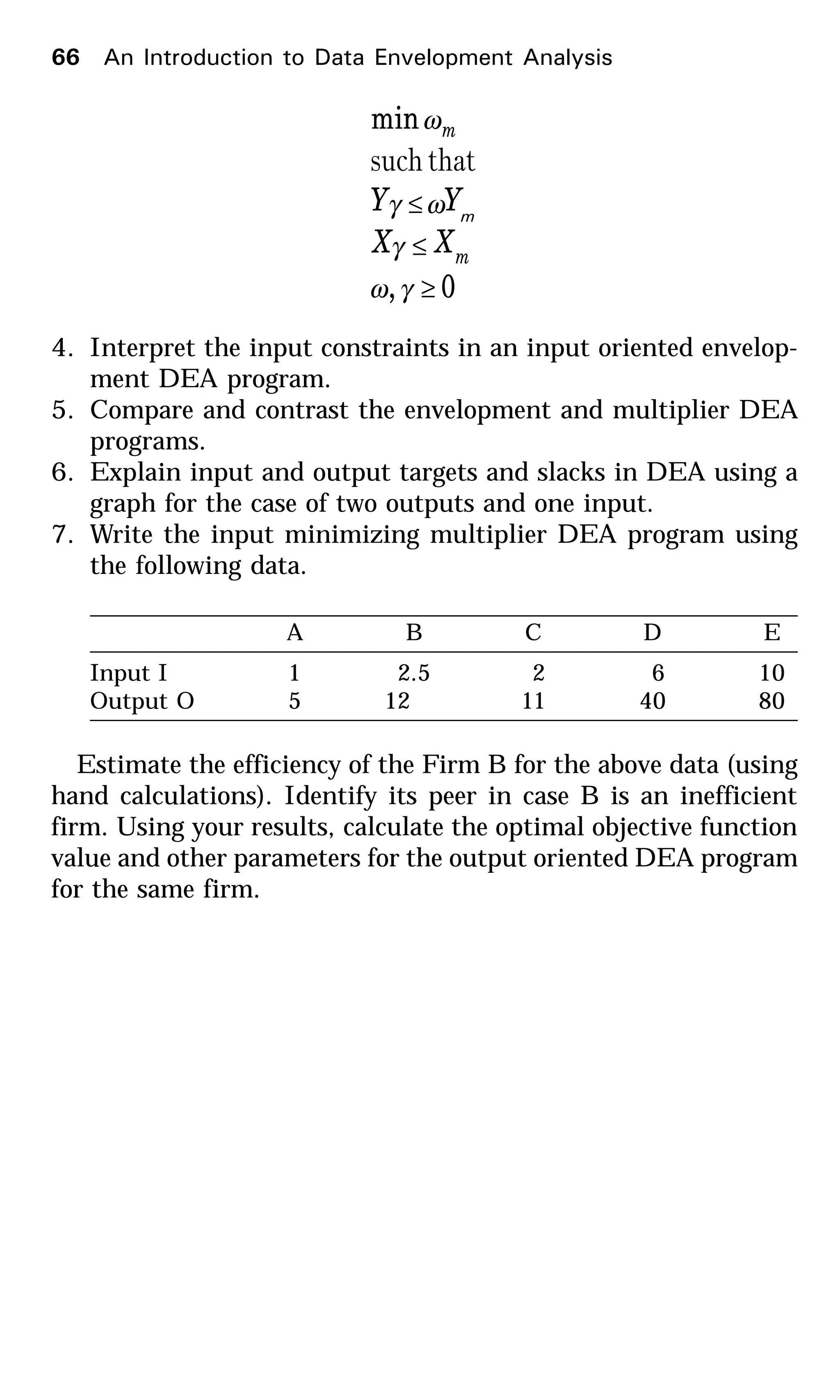
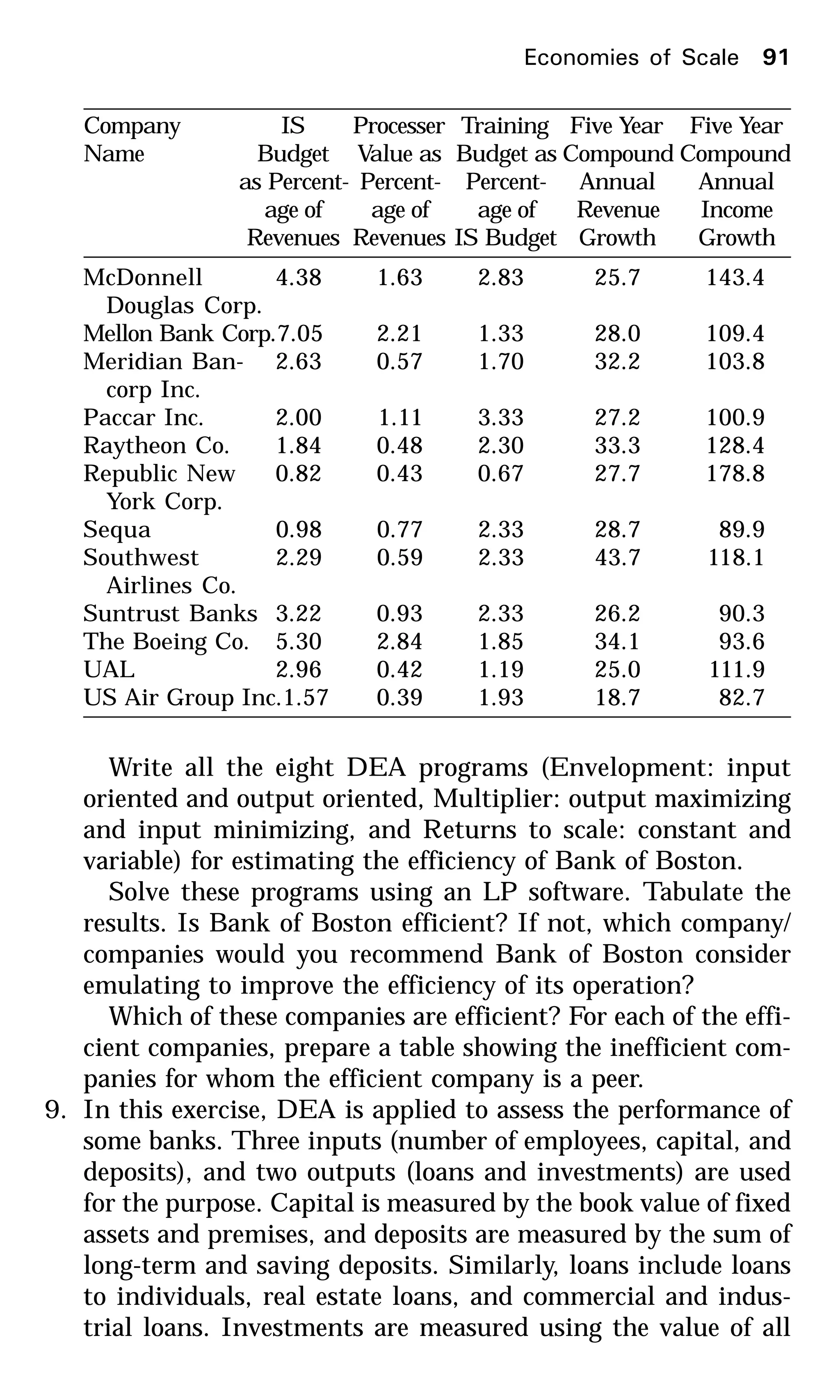
![174 An Introduction to Data Envelopment Analysis
effectively between efficient and inefficient DMUs.
However, there are many examples in the literature
where DEA has been used with small sample sizes.
t The sample size should be at least 2 or 3 times
larger than the sum of the number of inputs and
outputs.
7.1.2 Selection of Inputs and Outputs
A main difficulty in any application of DEA is in the selection of
inputs and outputs. The criteria of selection of these inputs and
outputs are quite subjective. There is no specific rule in deter-
mining the procedure for selection of inputs and outputs. However,
some guidelines may be suggested, and are discussed below.
A DEA study should start with an exhaustive, initial list of
inputs and outputs that are considered relevant for the study. At
this stage, all the inputs and outputs that have a bearing on the
performance of the DMUs to be analyzed should be listed. Screen-
ing procedures, which may be quantitative (e.g., statistical) or
qualitative (simply judgemental, using expert advice or using
methods such as the Analytic Hierarchy Process [Saaty 1980]),
may be used to pick up the most important inputs and outputs
and, therefore reducing the total number to a reasonable level.
For the purpose of this filtering, questions such as the following
may help:
(a) Is the input or output related to one or more of the objec-
tives of the DEA study?
(b) Does the input or output identify the characteristics of
the DMUs that are not captured by other inputs or out-
puts?
Normally, inputs are defined as resources utilized by the DMUs
or conditions affecting the performance of DMUs, while outputs
are the benefits generated as a result of the operation of the DMUs.
However, sometimes it may become difficult to classify a particular
factor as input or output, especially when the factor can be inter-
preted either as input or as output. In such cases, one way of
classifying the factor to check whether DMUs recording higher
performance in terms of that factor is considered more efficient](https://image.slidesharecdn.com/anintroductiontodea-180619020626/75/An-introduction-to-dea-175-2048.jpg)