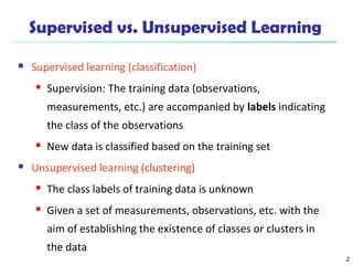
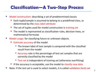
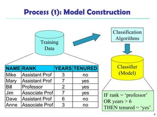
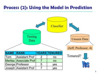
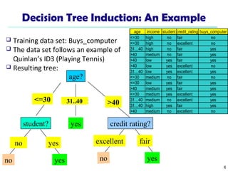
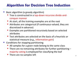
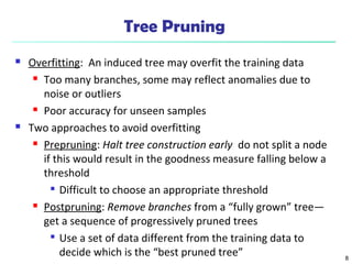
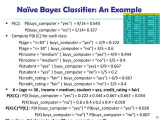
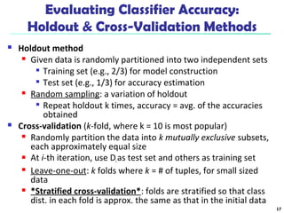
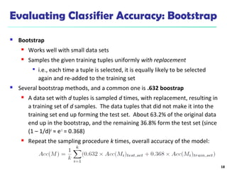
1
Module 4
Classification
By
Ms. Ankita Kadu
2
Supervised vs. Unsupervised Learning
 Supervised learning (classification)
 Supervision: The training data (observations,
measurements, etc.) are accompanied by labels indicating
the class of the observations
 New data is classified based on the training set
 Unsupervised learning (clustering)
 The class labels of training data is unknown
 Given a set of measurements, observations, etc. with the
aim of establishing the existence of classes or clusters in
the data
3
Classification—A Two-Step Process
 Model construction: describing a set of predetermined classes
 Each tuple/sample is assumed to belong to a predefined class, as
determined by the class label attribute
 The set of tuples used for model construction is training set
 The model is represented as classification rules, decision trees, or
mathematical formulae
 Model usage: for classifying future or unknown objects
 Estimate accuracy of the model

The known label of test sample is compared with the classified
result from the model

Accuracy rate is the percentage of test set samples that are
correctly classified by the model

Test set is independent of training set (otherwise overfitting)
 If the accuracy is acceptable, use the model to classify new data
 Note: If the test set is used to select models, it is called validation (test) set
4
Process (1): Model Construction
Training
Data
NAME RANK YEARS TENURED
Mike Assistant Prof 3 no
Mary Assistant Prof 7 yes
Bill Professor 2 yes
Jim Associate Prof 7 yes
Dave Assistant Prof 6 no
Anne Associate Prof 3 no
Classification
Algorithms
IF rank = ‘professor’
OR years > 6
THEN tenured = ‘yes’
Classifier
(Model)
5
Process (2): Using the Model in Prediction
Classifier
Testing
Data
NAME RANK YEARS TENURED
Tom Assistant Prof 2 no
Merlisa Associate Prof 7 no
George Professor 5 yes
Joseph Assistant Prof 7 yes
Unseen Data
(Jeff, Professor, 4)
Tenured?
6
Decision Tree Induction: An Example
age?
overcast
student? credit rating?
<=30 >40
no yes yes
yes
31..40
no
fairexcellentyesno
age income student credit_rating buys_computer
<=30 high no fair no
<=30 high no excellent no
31…40 high no fair yes
>40 medium no fair yes
>40 low yes fair yes
>40 low yes excellent no
31…40 low yes excellent yes
<=30 medium no fair no
<=30 low yes fair yes
>40 medium yes fair yes
<=30 medium yes excellent yes
31…40 medium no excellent yes
31…40 high yes fair yes
>40 medium no excellent no
 Training data set: Buys_computer
 The data set follows an example of
Quinlan’s ID3 (Playing Tennis)
 Resulting tree:
7
Algorithm for Decision Tree Induction
 Basic algorithm (a greedy algorithm)
 Tree is constructed in a top-down recursive divide-and-
conquer manner
 At start, all the training examples are at the root
 Attributes are categorical (if continuous-valued, they are
discretized in advance)
 Examples are partitioned recursively based on selected
attributes
 Test attributes are selected on the basis of a heuristic or
statistical measure (e.g., information gain)
 Conditions for stopping partitioning
 All samples for a given node belong to the same class
 There are no remaining attributes for further partitioning –
majority voting is employed for classifying the leaf
 There are no samples left
8
Tree Pruning
 Overfitting: An induced tree may overfit the training data
 Too many branches, some may reflect anomalies due to
noise or outliers
 Poor accuracy for unseen samples
 Two approaches to avoid overfitting
 Prepruning: Halt tree construction early do not split a node
if this would result in the goodness measure falling below a
threshold

Difficult to choose an appropriate threshold
 Postpruning: Remove branches from a “fully grown” tree—
get a sequence of progressively pruned trees

Use a set of data different from the training data to
decide which is the “best pruned tree”
9
Bayesian Classification: Why?
 A statistical classifier: performs probabilistic prediction, i.e.,
predicts class membership probabilities
 Foundation: Based on Bayes’ Theorem.
 Performance: A simple Bayesian classifier, naïve Bayesian
classifier, has comparable performance with decision tree and
selected neural network classifiers
 Incremental: Each training example can incrementally
increase/decrease the probability that a hypothesis is correct —
prior knowledge can be combined with observed data
 Standard: Even when Bayesian methods are computationally
intractable, they can provide a standard of optimal decision
making against which other methods can be measured
10
Bayes’ Theorem: Basics
 Total probability Theorem:
 Bayes’ Theorem:
 Let X be a data sample (“evidence”): class label is unknown
 Let H be a hypothesis that X belongs to class C
 Classification is to determine P(H|X), (i.e., posteriori probability): the
probability that the hypothesis holds given the observed data sample X
 P(H) (prior probability): the initial probability

E.g., X will buy computer, regardless of age, income, …
 P(X): probability that sample data is observed
 P(X|H) (likelihood): the probability of observing the sample X, given that
the hypothesis holds
)()
1
|()(
i
AP
M
i i
ABPBP ∑
=
=
)(/)()|(
)(
)()|()|( XX
X
XX PHPHP
P
HPHPHP ×==
11
Prediction Based on Bayes’ Theorem
 Given training data X, posteriori probability of a hypothesis H,
P(H|X), follows the Bayes’ theorem
 Informally, this can be viewed as
posteriori = likelihood x prior/evidence
 Predicts X belongs to Ci iff the probability P(Ci|X) is the highest
among all the P(Ck|X) for all the k classes
 Practical difficulty: It requires initial knowledge of many
probabilities, involving significant computational cost
)(/)()|(
)(
)()|()|( XX
X
XX PHPHP
P
HPHPHP ×==
12
Naïve Bayes Classifier: Training Dataset
Class:
C1:buys_computer = ‘yes’
C2:buys_computer = ‘no’
Data to be classified:
X = (age <=30,
Income = medium,
Student = yes
Credit_rating = Fair)
age income studentcredit_ratingbuys_compute
<=30 high no fair no
<=30 high no excellent no
31…40 high no fair yes
>40 medium no fair yes
>40 low yes fair yes
>40 low yes excellent no
31…40 low yes excellent yes
<=30 medium no fair no
<=30 low yes fair yes
>40 medium yes fair yes
<=30 medium yes excellent yes
31…40 medium no excellent yes
31…40 high yes fair yes
>40 medium no excellent no
13
Naïve Bayes Classifier: An Example
 P(Ci): P(buys_computer = “yes”) = 9/14 = 0.643
P(buys_computer = “no”) = 5/14= 0.357
 Compute P(X|Ci) for each class
P(age = “<=30” | buys_computer = “yes”) = 2/9 = 0.222
P(age = “<= 30” | buys_computer = “no”) = 3/5 = 0.6
P(income = “medium” | buys_computer = “yes”) = 4/9 = 0.444
P(income = “medium” | buys_computer = “no”) = 2/5 = 0.4
P(student = “yes” | buys_computer = “yes) = 6/9 = 0.667
P(student = “yes” | buys_computer = “no”) = 1/5 = 0.2
P(credit_rating = “fair” | buys_computer = “yes”) = 6/9 = 0.667
P(credit_rating = “fair” | buys_computer = “no”) = 2/5 = 0.4
 X = (age <= 30 , income = medium, student = yes, credit_rating = fair)
P(X|Ci) : P(X|buys_computer = “yes”) = 0.222 x 0.444 x 0.667 x 0.667 = 0.044
P(X|buys_computer = “no”) = 0.6 x 0.4 x 0.2 x 0.4 = 0.019
P(X|Ci)*P(Ci) : P(X|buys_computer = “yes”) * P(buys_computer = “yes”) = 0.028
P(X|buys_computer = “no”) * P(buys_computer = “no”) = 0.007
age income studentcredit_ratingbuys_comp
<=30 high no fair no
<=30 high no excellent no
31…40 high no fair yes
>40 medium no fair yes
>40 low yes fair yes
>40 low yes excellent no
31…40 low yes excellent yes
<=30 medium no fair no
<=30 low yes fair yes
>40 medium yes fair yes
<=30 medium yes excellent yes
31…40 medium no excellent yes
31…40 high yes fair yes
>40 medium no excellent no
14
Naïve Bayes Classifier
 Advantages
 Easy to implement
 Good results obtained in most of the cases
 Disadvantages
 Assumption: class conditional independence, therefore loss
of accuracy
 Practically, dependencies exist among variables

E.g., hospitals: patients: Profile: age, family history, etc.
Symptoms: fever, cough etc., Disease: lung cancer,
diabetes, etc.

Dependencies among these cannot be modeled by Naïve
Bayes Classifier
15
Using IF-THEN Rules for Classification
 Represent the knowledge in the form of IF-THEN rules
R: IF age = youth AND student = yes THEN buys_computer = yes
 Rule antecedent/precondition vs. rule consequent
 Assessment of a rule: coverage and accuracy
 ncovers= # of tuples covered by R
 ncorrect= # of tuples correctly classified by R
coverage(R) = ncovers/|D| /* D: training data set */
accuracy(R) = ncorrect/ ncovers
16
age?
student? credit rating?
<=30 >40
no yes yes
yes
31..40
no
fairexcellentyesno
 Example: Rule extraction from our buys_computer decision-tree
IF age = young AND student = no THEN buys_computer = no
IF age = young AND student = yes THEN buys_computer = yes
IF age = mid-age THEN buys_computer = yes
IF age = old AND credit_rating = excellent THEN buys_computer = no
IF age = old AND credit_rating = fair THEN buys_computer = yes
Rule Extraction from a Decision Tree
 Rules are easier to understand than large
trees
 One rule is created for each path from the
root to a leaf
 Each attribute-value pair along a path forms a
conjunction: the leaf holds the class
prediction
 Rules are mutually exclusive and exhaustive
Evaluating Classifier Accuracy:
Holdout & Cross-Validation Methods
 Holdout method
 Given data is randomly partitioned into two independent sets

Training set (e.g., 2/3) for model construction

Test set (e.g., 1/3) for accuracy estimation
 Random sampling: a variation of holdout

Repeat holdout k times, accuracy = avg. of the accuracies
obtained
 Cross-validation (k-fold, where k = 10 is most popular)
 Randomly partition the data into k mutually exclusive subsets,
each approximately equal size
 At i-th iteration, use Dias test set and others as training set
 Leave-one-out: k folds where k = # of tuples, for small sized
data
 *Stratified cross-validation*: folds are stratified so that class
dist. in each fold is approx. the same as that in the initial data
17
Evaluating Classifier Accuracy: Bootstrap
 Bootstrap
 Works well with small data sets
 Samples the given training tuples uniformly with replacement

i.e., each time a tuple is selected, it is equally likely to be selected
again and re-added to the training set
 Several bootstrap methods, and a common one is .632 boostrap
 A data set with d tuples is sampled d times, with replacement, resulting in
a training set of d samples. The data tuples that did not make it into the
training set end up forming the test set. About 63.2% of the original data
end up in the bootstrap, and the remaining 36.8% form the test set (since
(1 – 1/d)d
≈ e-1
= 0.368)
 Repeat the sampling procedure k times, overall accuracy of the model:
18

Classification

  • 1.
  • 2.
    2 Supervised vs. UnsupervisedLearning  Supervised learning (classification)  Supervision: The training data (observations, measurements, etc.) are accompanied by labels indicating the class of the observations  New data is classified based on the training set  Unsupervised learning (clustering)  The class labels of training data is unknown  Given a set of measurements, observations, etc. with the aim of establishing the existence of classes or clusters in the data
  • 3.
    3 Classification—A Two-Step Process Model construction: describing a set of predetermined classes  Each tuple/sample is assumed to belong to a predefined class, as determined by the class label attribute  The set of tuples used for model construction is training set  The model is represented as classification rules, decision trees, or mathematical formulae  Model usage: for classifying future or unknown objects  Estimate accuracy of the model  The known label of test sample is compared with the classified result from the model  Accuracy rate is the percentage of test set samples that are correctly classified by the model  Test set is independent of training set (otherwise overfitting)  If the accuracy is acceptable, use the model to classify new data  Note: If the test set is used to select models, it is called validation (test) set
  • 4.
    4 Process (1): ModelConstruction Training Data NAME RANK YEARS TENURED Mike Assistant Prof 3 no Mary Assistant Prof 7 yes Bill Professor 2 yes Jim Associate Prof 7 yes Dave Assistant Prof 6 no Anne Associate Prof 3 no Classification Algorithms IF rank = ‘professor’ OR years > 6 THEN tenured = ‘yes’ Classifier (Model)
  • 5.
    5 Process (2): Usingthe Model in Prediction Classifier Testing Data NAME RANK YEARS TENURED Tom Assistant Prof 2 no Merlisa Associate Prof 7 no George Professor 5 yes Joseph Assistant Prof 7 yes Unseen Data (Jeff, Professor, 4) Tenured?
  • 6.
    6 Decision Tree Induction:An Example age? overcast student? credit rating? <=30 >40 no yes yes yes 31..40 no fairexcellentyesno age income student credit_rating buys_computer <=30 high no fair no <=30 high no excellent no 31…40 high no fair yes >40 medium no fair yes >40 low yes fair yes >40 low yes excellent no 31…40 low yes excellent yes <=30 medium no fair no <=30 low yes fair yes >40 medium yes fair yes <=30 medium yes excellent yes 31…40 medium no excellent yes 31…40 high yes fair yes >40 medium no excellent no  Training data set: Buys_computer  The data set follows an example of Quinlan’s ID3 (Playing Tennis)  Resulting tree:
  • 7.
    7 Algorithm for DecisionTree Induction  Basic algorithm (a greedy algorithm)  Tree is constructed in a top-down recursive divide-and- conquer manner  At start, all the training examples are at the root  Attributes are categorical (if continuous-valued, they are discretized in advance)  Examples are partitioned recursively based on selected attributes  Test attributes are selected on the basis of a heuristic or statistical measure (e.g., information gain)  Conditions for stopping partitioning  All samples for a given node belong to the same class  There are no remaining attributes for further partitioning – majority voting is employed for classifying the leaf  There are no samples left
  • 8.
    8 Tree Pruning  Overfitting:An induced tree may overfit the training data  Too many branches, some may reflect anomalies due to noise or outliers  Poor accuracy for unseen samples  Two approaches to avoid overfitting  Prepruning: Halt tree construction early do not split a node if this would result in the goodness measure falling below a threshold  Difficult to choose an appropriate threshold  Postpruning: Remove branches from a “fully grown” tree— get a sequence of progressively pruned trees  Use a set of data different from the training data to decide which is the “best pruned tree”
  • 9.
    9 Bayesian Classification: Why? A statistical classifier: performs probabilistic prediction, i.e., predicts class membership probabilities  Foundation: Based on Bayes’ Theorem.  Performance: A simple Bayesian classifier, naïve Bayesian classifier, has comparable performance with decision tree and selected neural network classifiers  Incremental: Each training example can incrementally increase/decrease the probability that a hypothesis is correct — prior knowledge can be combined with observed data  Standard: Even when Bayesian methods are computationally intractable, they can provide a standard of optimal decision making against which other methods can be measured
  • 10.
    10 Bayes’ Theorem: Basics Total probability Theorem:  Bayes’ Theorem:  Let X be a data sample (“evidence”): class label is unknown  Let H be a hypothesis that X belongs to class C  Classification is to determine P(H|X), (i.e., posteriori probability): the probability that the hypothesis holds given the observed data sample X  P(H) (prior probability): the initial probability  E.g., X will buy computer, regardless of age, income, …  P(X): probability that sample data is observed  P(X|H) (likelihood): the probability of observing the sample X, given that the hypothesis holds )() 1 |()( i AP M i i ABPBP ∑ = = )(/)()|( )( )()|()|( XX X XX PHPHP P HPHPHP ×==
  • 11.
    11 Prediction Based onBayes’ Theorem  Given training data X, posteriori probability of a hypothesis H, P(H|X), follows the Bayes’ theorem  Informally, this can be viewed as posteriori = likelihood x prior/evidence  Predicts X belongs to Ci iff the probability P(Ci|X) is the highest among all the P(Ck|X) for all the k classes  Practical difficulty: It requires initial knowledge of many probabilities, involving significant computational cost )(/)()|( )( )()|()|( XX X XX PHPHP P HPHPHP ×==
  • 12.
    12 Naïve Bayes Classifier:Training Dataset Class: C1:buys_computer = ‘yes’ C2:buys_computer = ‘no’ Data to be classified: X = (age <=30, Income = medium, Student = yes Credit_rating = Fair) age income studentcredit_ratingbuys_compute <=30 high no fair no <=30 high no excellent no 31…40 high no fair yes >40 medium no fair yes >40 low yes fair yes >40 low yes excellent no 31…40 low yes excellent yes <=30 medium no fair no <=30 low yes fair yes >40 medium yes fair yes <=30 medium yes excellent yes 31…40 medium no excellent yes 31…40 high yes fair yes >40 medium no excellent no
  • 13.
    13 Naïve Bayes Classifier:An Example  P(Ci): P(buys_computer = “yes”) = 9/14 = 0.643 P(buys_computer = “no”) = 5/14= 0.357  Compute P(X|Ci) for each class P(age = “<=30” | buys_computer = “yes”) = 2/9 = 0.222 P(age = “<= 30” | buys_computer = “no”) = 3/5 = 0.6 P(income = “medium” | buys_computer = “yes”) = 4/9 = 0.444 P(income = “medium” | buys_computer = “no”) = 2/5 = 0.4 P(student = “yes” | buys_computer = “yes) = 6/9 = 0.667 P(student = “yes” | buys_computer = “no”) = 1/5 = 0.2 P(credit_rating = “fair” | buys_computer = “yes”) = 6/9 = 0.667 P(credit_rating = “fair” | buys_computer = “no”) = 2/5 = 0.4  X = (age <= 30 , income = medium, student = yes, credit_rating = fair) P(X|Ci) : P(X|buys_computer = “yes”) = 0.222 x 0.444 x 0.667 x 0.667 = 0.044 P(X|buys_computer = “no”) = 0.6 x 0.4 x 0.2 x 0.4 = 0.019 P(X|Ci)*P(Ci) : P(X|buys_computer = “yes”) * P(buys_computer = “yes”) = 0.028 P(X|buys_computer = “no”) * P(buys_computer = “no”) = 0.007 age income studentcredit_ratingbuys_comp <=30 high no fair no <=30 high no excellent no 31…40 high no fair yes >40 medium no fair yes >40 low yes fair yes >40 low yes excellent no 31…40 low yes excellent yes <=30 medium no fair no <=30 low yes fair yes >40 medium yes fair yes <=30 medium yes excellent yes 31…40 medium no excellent yes 31…40 high yes fair yes >40 medium no excellent no
  • 14.
    14 Naïve Bayes Classifier Advantages  Easy to implement  Good results obtained in most of the cases  Disadvantages  Assumption: class conditional independence, therefore loss of accuracy  Practically, dependencies exist among variables  E.g., hospitals: patients: Profile: age, family history, etc. Symptoms: fever, cough etc., Disease: lung cancer, diabetes, etc.  Dependencies among these cannot be modeled by Naïve Bayes Classifier
  • 15.
    15 Using IF-THEN Rulesfor Classification  Represent the knowledge in the form of IF-THEN rules R: IF age = youth AND student = yes THEN buys_computer = yes  Rule antecedent/precondition vs. rule consequent  Assessment of a rule: coverage and accuracy  ncovers= # of tuples covered by R  ncorrect= # of tuples correctly classified by R coverage(R) = ncovers/|D| /* D: training data set */ accuracy(R) = ncorrect/ ncovers
  • 16.
    16 age? student? credit rating? <=30>40 no yes yes yes 31..40 no fairexcellentyesno  Example: Rule extraction from our buys_computer decision-tree IF age = young AND student = no THEN buys_computer = no IF age = young AND student = yes THEN buys_computer = yes IF age = mid-age THEN buys_computer = yes IF age = old AND credit_rating = excellent THEN buys_computer = no IF age = old AND credit_rating = fair THEN buys_computer = yes Rule Extraction from a Decision Tree  Rules are easier to understand than large trees  One rule is created for each path from the root to a leaf  Each attribute-value pair along a path forms a conjunction: the leaf holds the class prediction  Rules are mutually exclusive and exhaustive
  • 17.
    Evaluating Classifier Accuracy: Holdout& Cross-Validation Methods  Holdout method  Given data is randomly partitioned into two independent sets  Training set (e.g., 2/3) for model construction  Test set (e.g., 1/3) for accuracy estimation  Random sampling: a variation of holdout  Repeat holdout k times, accuracy = avg. of the accuracies obtained  Cross-validation (k-fold, where k = 10 is most popular)  Randomly partition the data into k mutually exclusive subsets, each approximately equal size  At i-th iteration, use Dias test set and others as training set  Leave-one-out: k folds where k = # of tuples, for small sized data  *Stratified cross-validation*: folds are stratified so that class dist. in each fold is approx. the same as that in the initial data 17
  • 18.
    Evaluating Classifier Accuracy:Bootstrap  Bootstrap  Works well with small data sets  Samples the given training tuples uniformly with replacement  i.e., each time a tuple is selected, it is equally likely to be selected again and re-added to the training set  Several bootstrap methods, and a common one is .632 boostrap  A data set with d tuples is sampled d times, with replacement, resulting in a training set of d samples. The data tuples that did not make it into the training set end up forming the test set. About 63.2% of the original data end up in the bootstrap, and the remaining 36.8% form the test set (since (1 – 1/d)d ≈ e-1 = 0.368)  Repeat the sampling procedure k times, overall accuracy of the model: 18