4_22865_IS465_2019_1__2_1_08ClassBasic.ppt

1
Data Mining:
Concepts and Techniques
(3rd
ed.)
— Chapter 8 —
Jiawei Han, Micheline Kamber, and Jian Pei
University of Illinois at Urbana-Champaign &
Simon Fraser University
©2011 Han, Kamber & Pei. All rights reserved.

2
Chapter 8. Classification: Basic Concepts
 Classification: Basic Concepts
 Decision Tree Induction
 Bayes Classification Methods
 Rule-Based Classification
 Model Evaluation and Selection
 Techniques to Improve Classification Accuracy:
Ensemble Methods
 Summary

3
Supervised vs. Unsupervised Learning
 Supervised learning (classification)
 Supervision: The training data (observations,
measurements, etc.) are accompanied by labels indicating
the class of the observations
 New data is classified based on the training set
 Unsupervised learning (clustering)

The class labels of training data is unknown

Given a set of measurements, observations, etc. with the
aim of establishing the existence of classes or clusters in the
data

4
 Classification
 predicts categorical class labels (discrete or nominal)
 classifies data (constructs a model) based on the training
set and the values (class labels) in a classifying attribute and
uses it in classifying new data
 Numeric Prediction
 models continuous-valued functions, i.e., predicts unknown
or missing values
 Typical applications
 Credit/loan approval:
 Medical diagnosis: if a tumor is cancerous or benign
 Fraud detection: if a transaction is fraudulent
 Web page categorization: which category it is
Prediction Problems: Classification vs.
Numeric Prediction

5
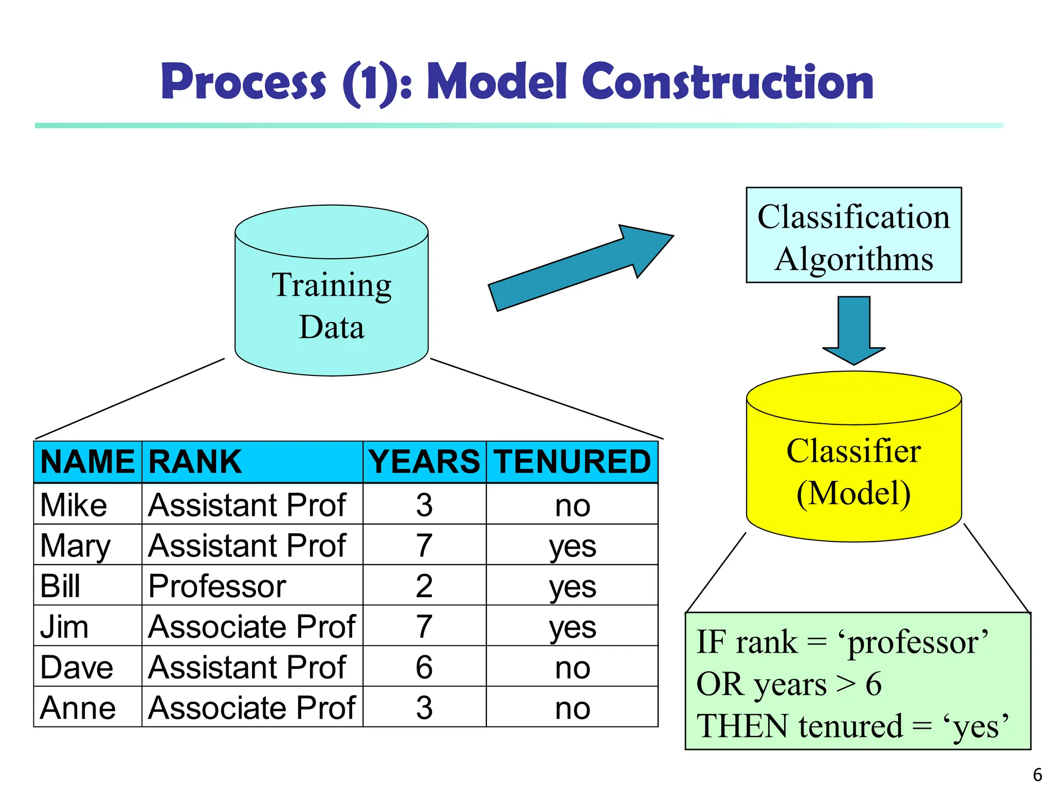
Classification—A Two-Step Process
 Model construction: describing a set of predetermined classes

Each tuple/sample is assumed to belong to a predefined class, as
determined by the class label attribute

The set of tuples used for model construction is training set
 The model is represented as classification rules, decision trees, or
mathematical formulae
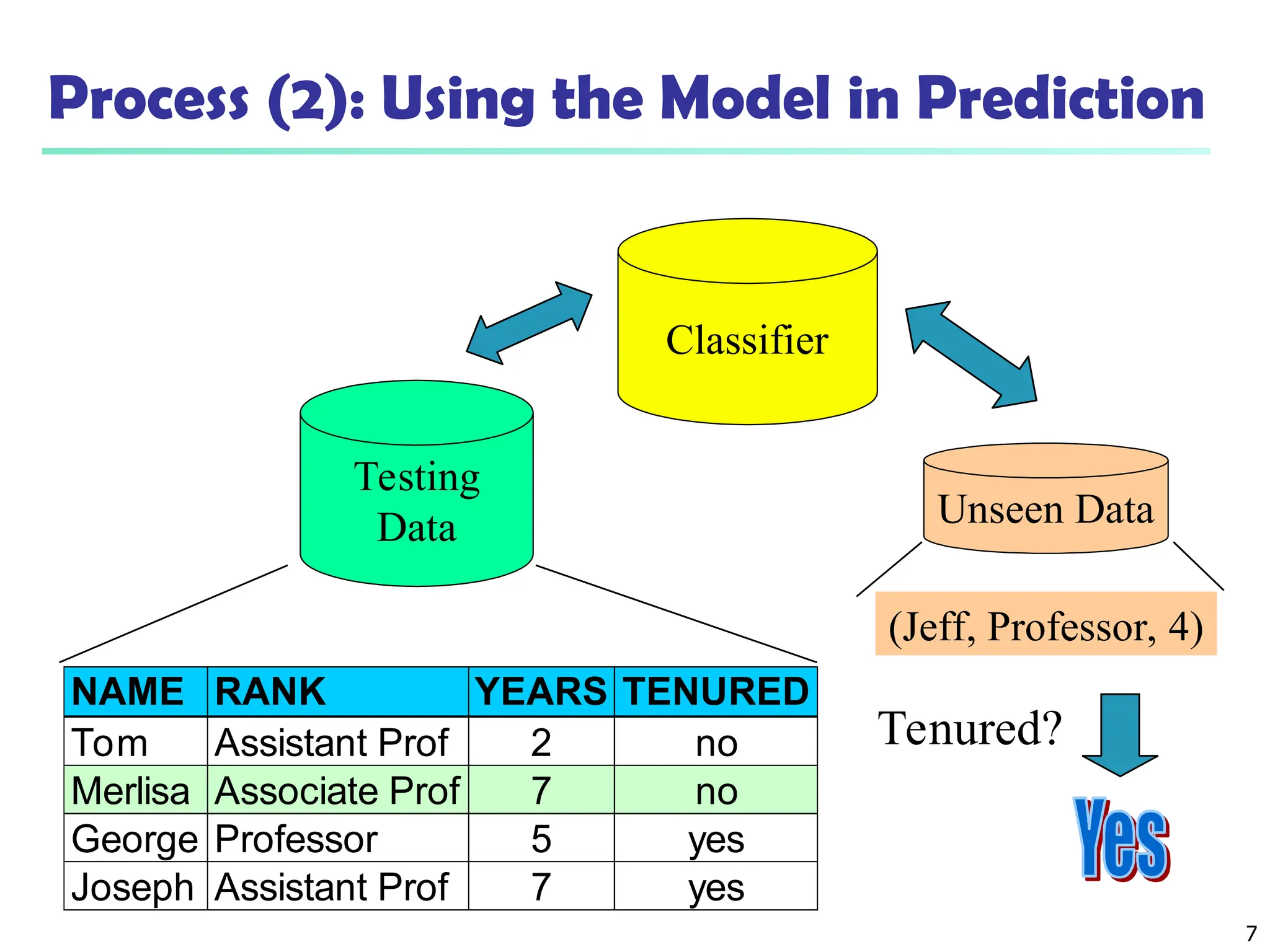
 Model usage: for classifying future or unknown objects
 Estimate accuracy of the model

The known label of test sample is compared with the classified result
from the model

Accuracy rate is the percentage of test set samples that are correctly
classified by the model

Test set is independent of training set (otherwise overfitting)

If the accuracy is acceptable, use the model to classify new data
 Note: If the test set is used to select models, it is called validation (test) set

6
Process (1): Model Construction
Training
Data
NAME RANK YEARS TENURED
Mike Assistant Prof 3 no
Mary Assistant Prof 7 yes
Bill Professor 2 yes
Jim Associate Prof 7 yes
Dave Assistant Prof 6 no
Anne Associate Prof 3 no
Classification
Algorithms
IF rank = ‘professor’
OR years > 6
THEN tenured = ‘yes’
Classifier
(Model)

7
Process (2): Using the Model in Prediction
Classifier
Testing
Data
NAME RANK YEARS TENURED
Tom Assistant Prof 2 no
Merlisa Associate Prof 7 no
George Professor 5 yes
Joseph Assistant Prof 7 yes
Unseen Data
(Jeff, Professor, 4)
Tenured?

8
Ensemble Methods
 Summary

9
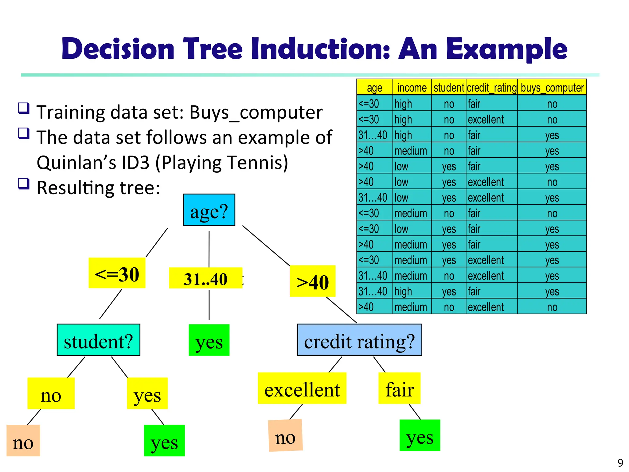
Decision Tree Induction: An Example
age?
overcast
student? credit rating?
<=30 >40
no yes yes
yes
31..40
no
fair
excellent
yes
no
age income student credit_rating buys_computer
<=30 high no fair no
<=30 high no excellent no
31…40 high no fair yes
>40 medium no fair yes
>40 low yes fair yes
>40 low yes excellent no
31…40 low yes excellent yes
<=30 medium no fair no
<=30 low yes fair yes
>40 medium yes fair yes
<=30 medium yes excellent yes
31…40 medium no excellent yes
31…40 high yes fair yes
>40 medium no excellent no
 Training data set: Buys_computer
 The data set follows an example of
Quinlan’s ID3 (Playing Tennis)
 Resulting tree:

10
Algorithm for Decision Tree Induction
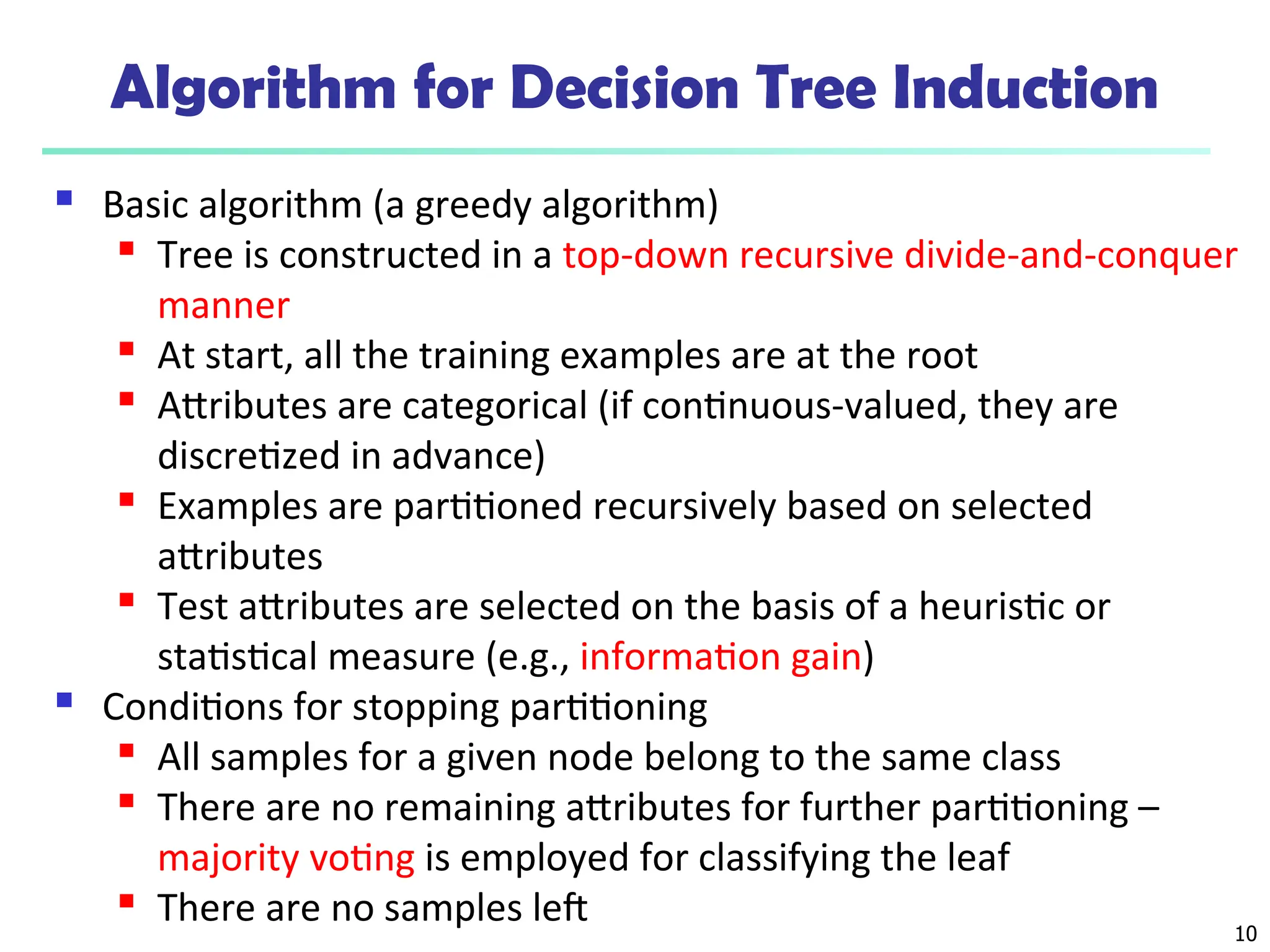
 Basic algorithm (a greedy algorithm)
 Tree is constructed in a top-down recursive divide-and-conquer
manner
 At start, all the training examples are at the root
 Attributes are categorical (if continuous-valued, they are
discretized in advance)
 Examples are partitioned recursively based on selected
attributes
 Test attributes are selected on the basis of a heuristic or
statistical measure (e.g., information gain)
 Conditions for stopping partitioning
 All samples for a given node belong to the same class
 There are no remaining attributes for further partitioning –
majority voting is employed for classifying the leaf
 There are no samples left

Brief Review of Entropy
11
m = 2

12
Attribute Selection Measure:
Information Gain (ID3/C4.5)
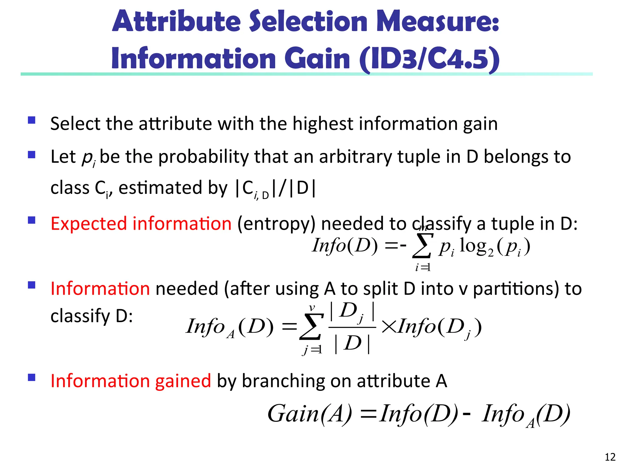
 Select the attribute with the highest information gain
 Let pi be the probability that an arbitrary tuple in D belongs to
class Ci, estimated by |Ci, D|/|D|
 Expected information (entropy) needed to classify a tuple in D:
 Information needed (after using A to split D into v partitions) to
classify D:
 Information gained by branching on attribute A
)
(
log
)
( 2
1
i
m
i
i p
p
D
Info 



)
(
|
|
|
|
)
(
1
j
v
j
j
A D
Info
D
D
D
Info 


(D)
Info
Info(D)
Gain(A) A



13
Attribute Selection: Information Gain
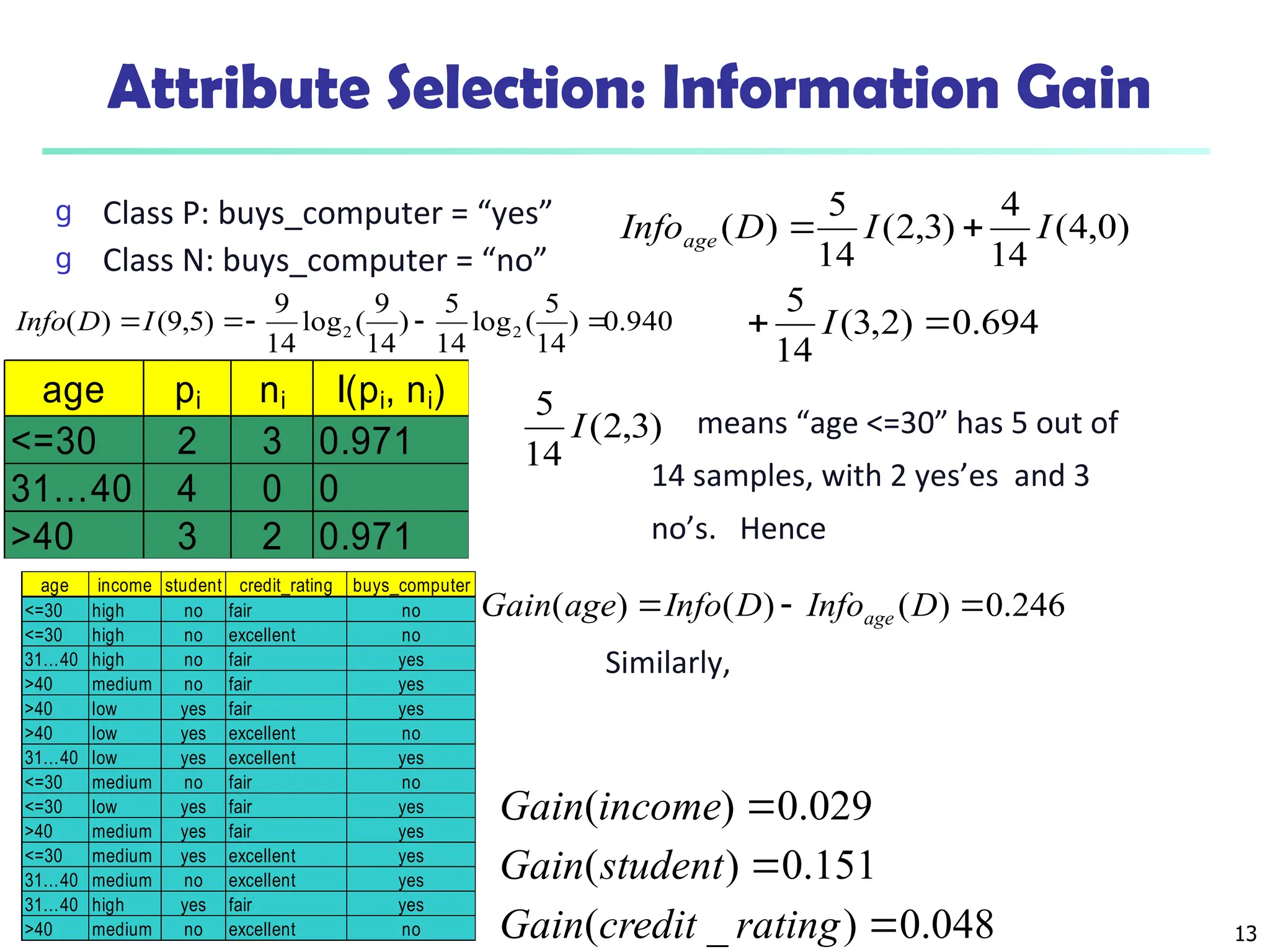
g Class P: buys_computer = “yes”
g Class N: buys_computer = “no”
means “age <=30” has 5 out of
14 samples, with 2 yes’es and 3
no’s. Hence
Similarly,
age pi ni I(pi, ni)
<=30 2 3 0.971
31…40 4 0 0
>40 3 2 0.971
694
.
0
)
2
,
3
(
14
5
)
0
,
4
(
14
4
)
3
,
2
(
14
5
)
(




I
I
I
D
Infoage
048
.
0
)
_
(
151
.
0
)
(
029
.
0
)
(



rating
credit
Gain
student
Gain
income
Gain
246
.
0
)
(
)
(
)
( 

 D
Info
D
Info
age
Gain age
age income student credit_rating buys_computer
)
3
,
2
(
14
5
I
940
.
0
)
14
5
(
log
14
5
)
14
9
(
log
14
9
)
5
,
9
(
)
( 2
2 



I
D
Info

14
Ensemble Methods
 Summary

15
Bayesian Classification: Why?
 A statistical classifier: performs probabilistic prediction, i.e.,
predicts class membership probabilities
 Foundation: Based on Bayes’ Theorem.
 Performance: A simple Bayesian classifier, naïve Bayesian
classifier, has comparable performance with decision tree and
selected neural network classifiers
 Incremental: Each training example can incrementally
increase/decrease the probability that a hypothesis is correct —
prior knowledge can be combined with observed data
 Standard: Even when Bayesian methods are computationally
intractable, they can provide a standard of optimal decision
making against which other methods can be measured

16
Bayes’ Theorem: Basics
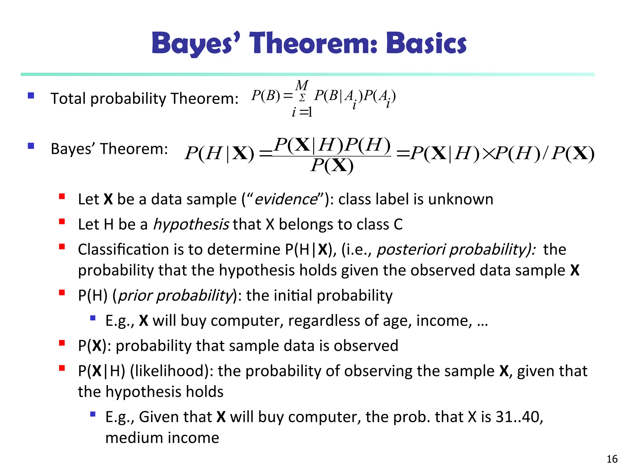
 Total probability Theorem:
 Bayes’ Theorem:
 Let X be a data sample (“evidence”): class label is unknown
 Let H be a hypothesis that X belongs to class C
 Classification is to determine P(H|X), (i.e., posteriori probability): the
probability that the hypothesis holds given the observed data sample X
 P(H) (prior probability): the initial probability

E.g., X will buy computer, regardless of age, income, …
 P(X): probability that sample data is observed
 P(X|H) (likelihood): the probability of observing the sample X, given that
the hypothesis holds

E.g., Given that X will buy computer, the prob. that X is 31..40,
medium income
)
(
)
1
|
(
)
(
i
A
P
M
i i
A
B
P
B
P 


)
(
/
)
(
)
|
(
)
(
)
(
)
|
(
)
|
( X
X
X
X
X P
H
P
H
P
P
H
P
H
P
H
P 



17
Prediction Based on Bayes’ Theorem
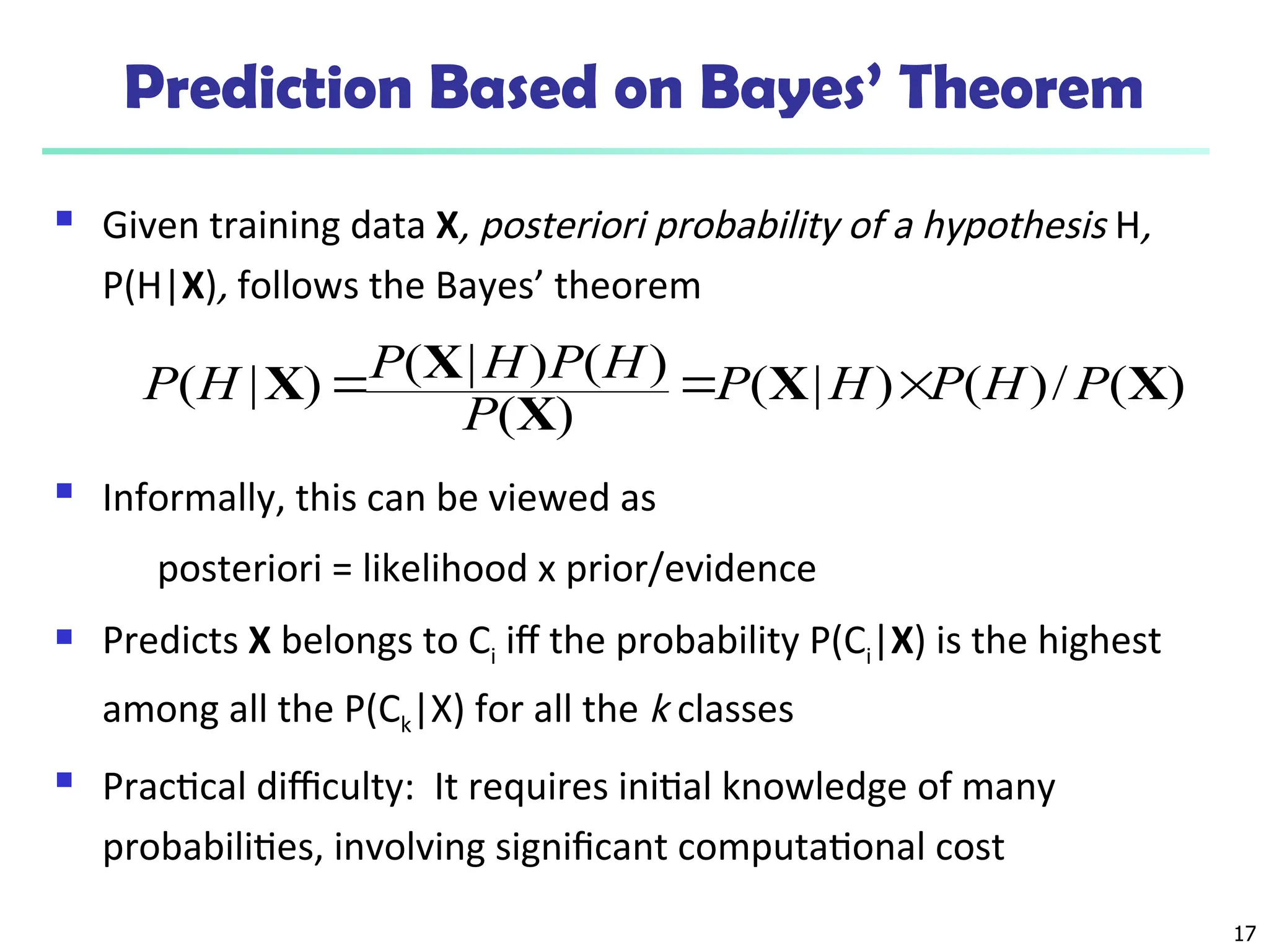
 Given training data X, posteriori probability of a hypothesis H,
P(H|X), follows the Bayes’ theorem
 Informally, this can be viewed as
posteriori = likelihood x prior/evidence
 Predicts X belongs to Ci iff the probability P(Ci|X) is the highest
among all the P(Ck|X) for all the k classes
 Practical difficulty: It requires initial knowledge of many
probabilities, involving significant computational cost
)
(
/
)
(
)
|
(
)
(
)
(
)
|
(
)
|
( X
X
X
X
X P
H
P
H
P
P
H
P
H
P
H
P 



18
Classification Is to Derive the Maximum Posteriori
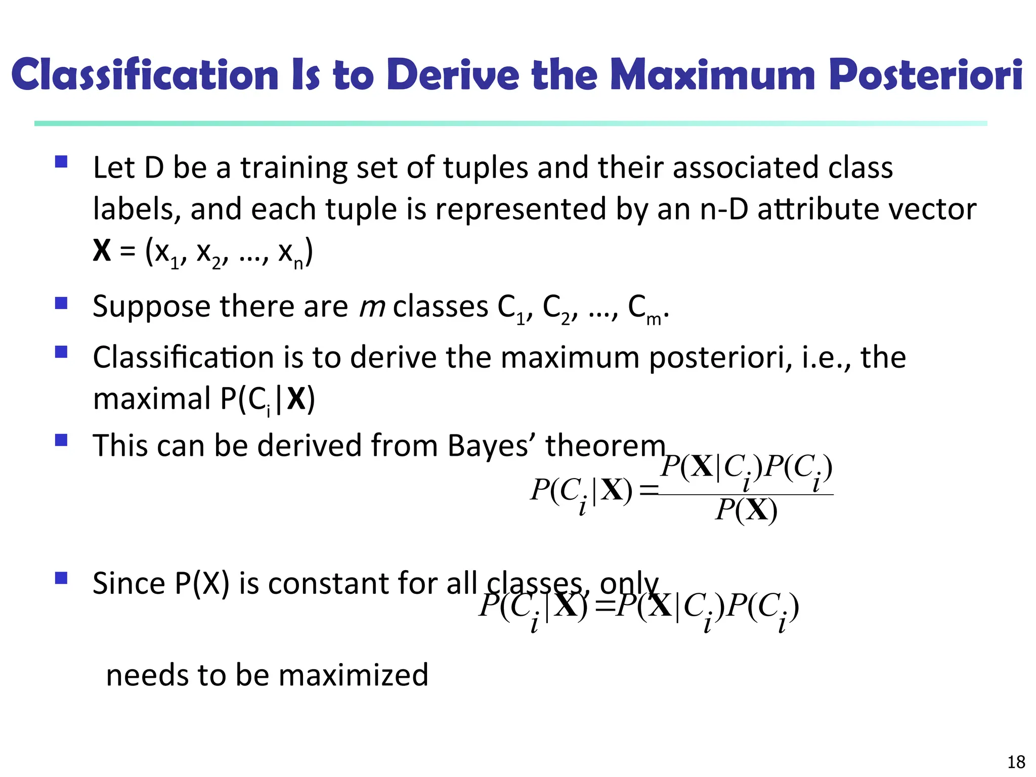
 Let D be a training set of tuples and their associated class
labels, and each tuple is represented by an n-D attribute vector
X = (x1, x2, …, xn)
 Suppose there are m classes C1, C2, …, Cm.
 Classification is to derive the maximum posteriori, i.e., the
maximal P(Ci|X)
 This can be derived from Bayes’ theorem
 Since P(X) is constant for all classes, only
needs to be maximized
)
(
)
(
)
|
(
)
|
(
X
X
X
P
i
C
P
i
C
P
i
C
P 
)
(
)
|
(
)
|
(
i
C
P
i
C
P
i
C
P X
X 

19
Naïve Bayes Classifier
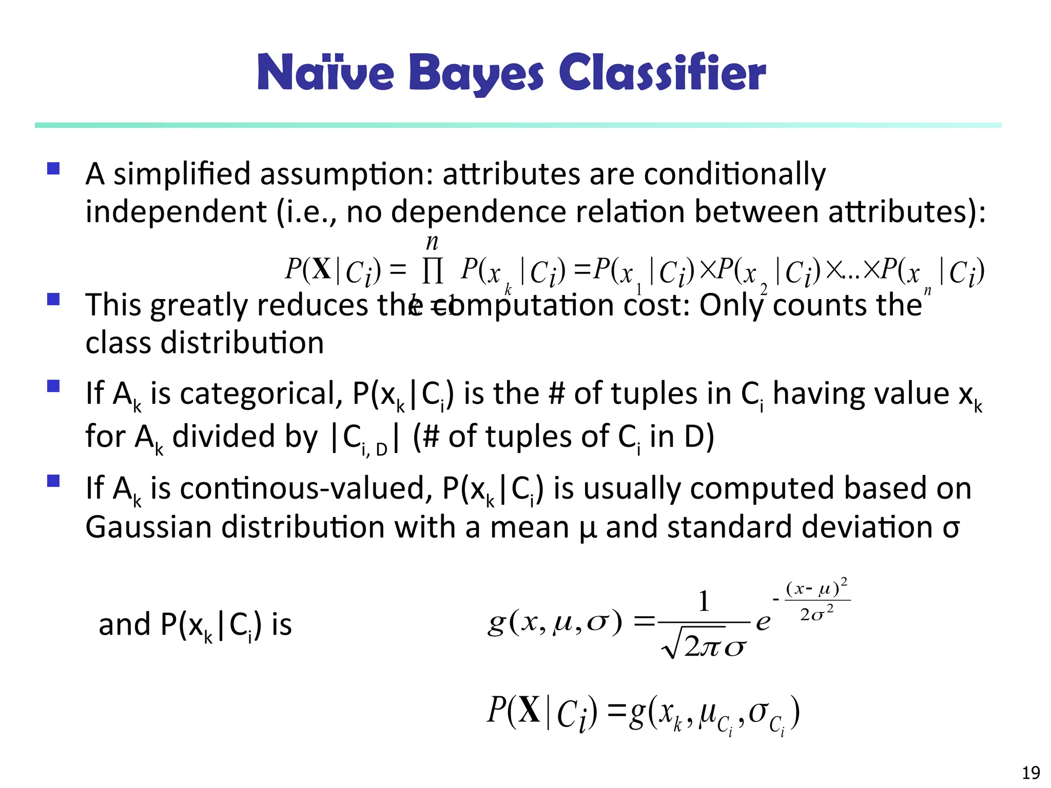
 A simplified assumption: attributes are conditionally
independent (i.e., no dependence relation between attributes):
 This greatly reduces the computation cost: Only counts the
class distribution
 If Ak is categorical, P(xk|Ci) is the # of tuples in Ci having value xk
for Ak divided by |Ci, D| (# of tuples of Ci in D)
 If Ak is continous-valued, P(xk|Ci) is usually computed based on
Gaussian distribution with a mean μ and standard deviation σ
and P(xk|Ci) is
)
|
(
...
)
|
(
)
|
(
1
)
|
(
)
|
(
2
1
Ci
x
P
Ci
x
P
Ci
x
P
n
k
Ci
x
P
Ci
P
n
k







X
2
2
2
)
(
2
1
)
,
,
( 








x
e
x
g
)
,
,
(
)
|
( i
i C
C
k
x
g
Ci
P 


X

20
Naïve Bayes Classifier: Training Dataset
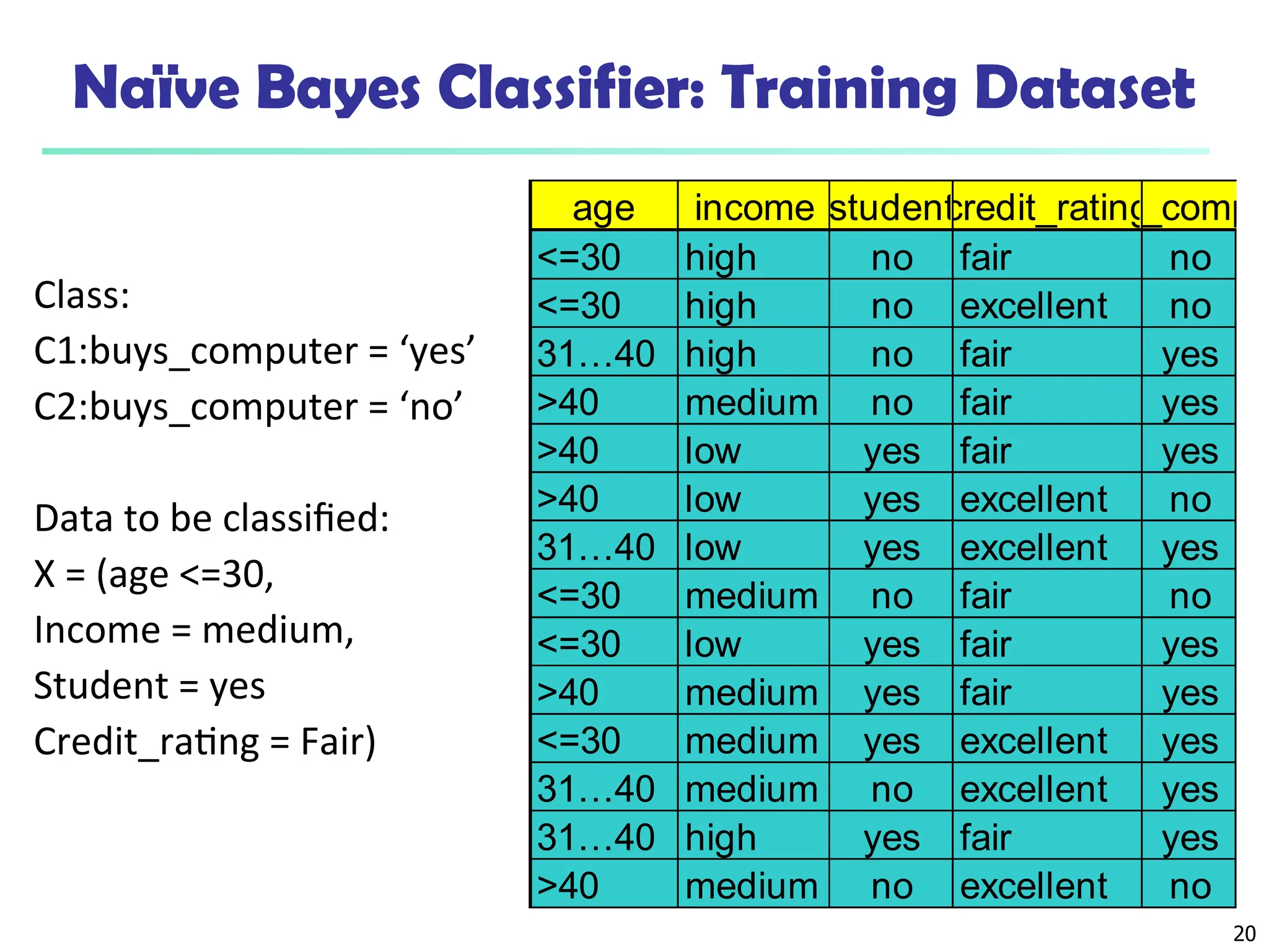
Class:
C1:buys_computer = ‘yes’
C2:buys_computer = ‘no’
Data to be classified:
X = (age <=30,
Income = medium,
Student = yes
Credit_rating = Fair)
age income student
credit_rating
buys_compu

21
Naïve Bayes Classifier: An Example
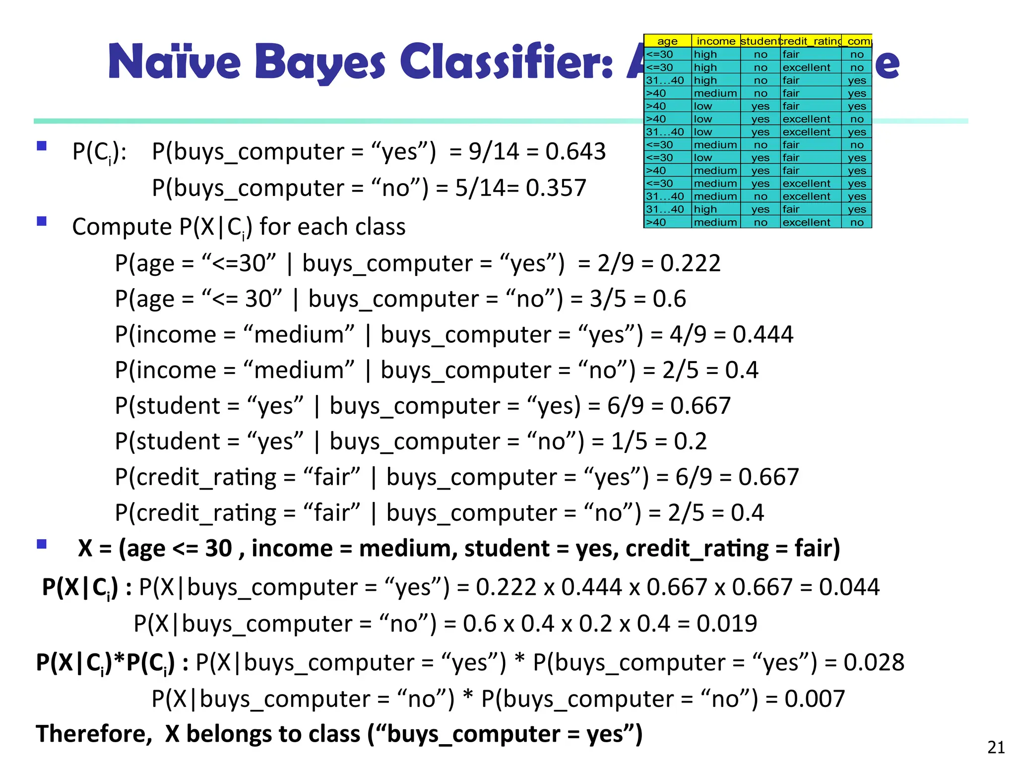
 P(Ci): P(buys_computer = “yes”) = 9/14 = 0.643
P(buys_computer = “no”) = 5/14= 0.357
 Compute P(X|Ci) for each class
P(age = “<=30” | buys_computer = “yes”) = 2/9 = 0.222
P(age = “<= 30” | buys_computer = “no”) = 3/5 = 0.6
P(income = “medium” | buys_computer = “yes”) = 4/9 = 0.444
P(income = “medium” | buys_computer = “no”) = 2/5 = 0.4
P(student = “yes” | buys_computer = “yes) = 6/9 = 0.667
P(student = “yes” | buys_computer = “no”) = 1/5 = 0.2
P(credit_rating = “fair” | buys_computer = “yes”) = 6/9 = 0.667
P(credit_rating = “fair” | buys_computer = “no”) = 2/5 = 0.4
 X = (age <= 30 , income = medium, student = yes, credit_rating = fair)
P(X|Ci) : P(X|buys_computer = “yes”) = 0.222 x 0.444 x 0.667 x 0.667 = 0.044
P(X|buys_computer = “no”) = 0.6 x 0.4 x 0.2 x 0.4 = 0.019
P(X|Ci)*P(Ci) : P(X|buys_computer = “yes”) * P(buys_computer = “yes”) = 0.028
P(X|buys_computer = “no”) * P(buys_computer = “no”) = 0.007
Therefore, X belongs to class (“buys_computer = yes”)
age income student
credit_rating
buys_computer

22
Avoiding the Zero-Probability Problem
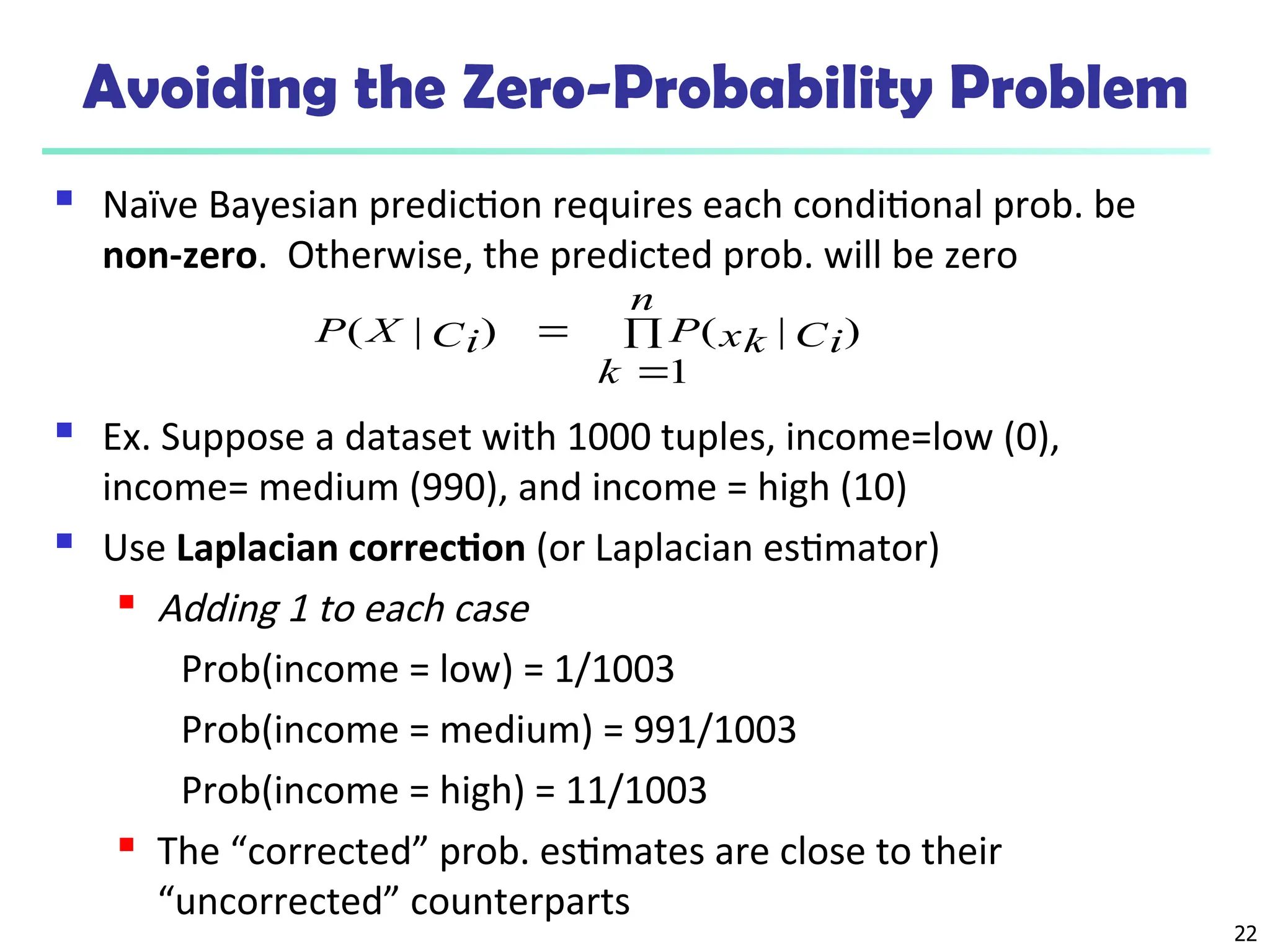
 Naïve Bayesian prediction requires each conditional prob. be
non-zero. Otherwise, the predicted prob. will be zero
 Ex. Suppose a dataset with 1000 tuples, income=low (0),
income= medium (990), and income = high (10)
 Use Laplacian correction (or Laplacian estimator)
 Adding 1 to each case
Prob(income = low) = 1/1003
Prob(income = medium) = 991/1003
Prob(income = high) = 11/1003

The “corrected” prob. estimates are close to their
“uncorrected” counterparts



n
k
Ci
xk
P
Ci
X
P
1
)
|
(
)
|
(

23
Naïve Bayes Classifier: Comments
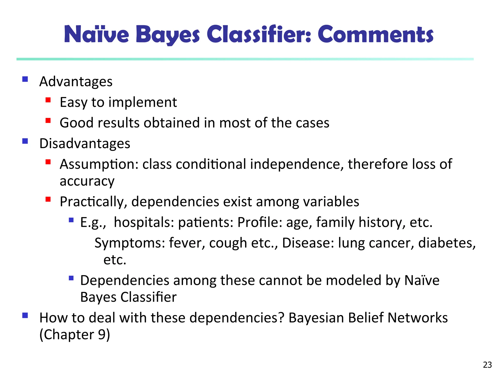
 Advantages
 Easy to implement
 Good results obtained in most of the cases
 Disadvantages
 Assumption: class conditional independence, therefore loss of
accuracy
 Practically, dependencies exist among variables

E.g., hospitals: patients: Profile: age, family history, etc.
Symptoms: fever, cough etc., Disease: lung cancer, diabetes,
etc.

Dependencies among these cannot be modeled by Naïve
Bayes Classifier
 How to deal with these dependencies? Bayesian Belief Networks
(Chapter 9)

24
Ensemble Methods
 Summary

Model Evaluation and Selection
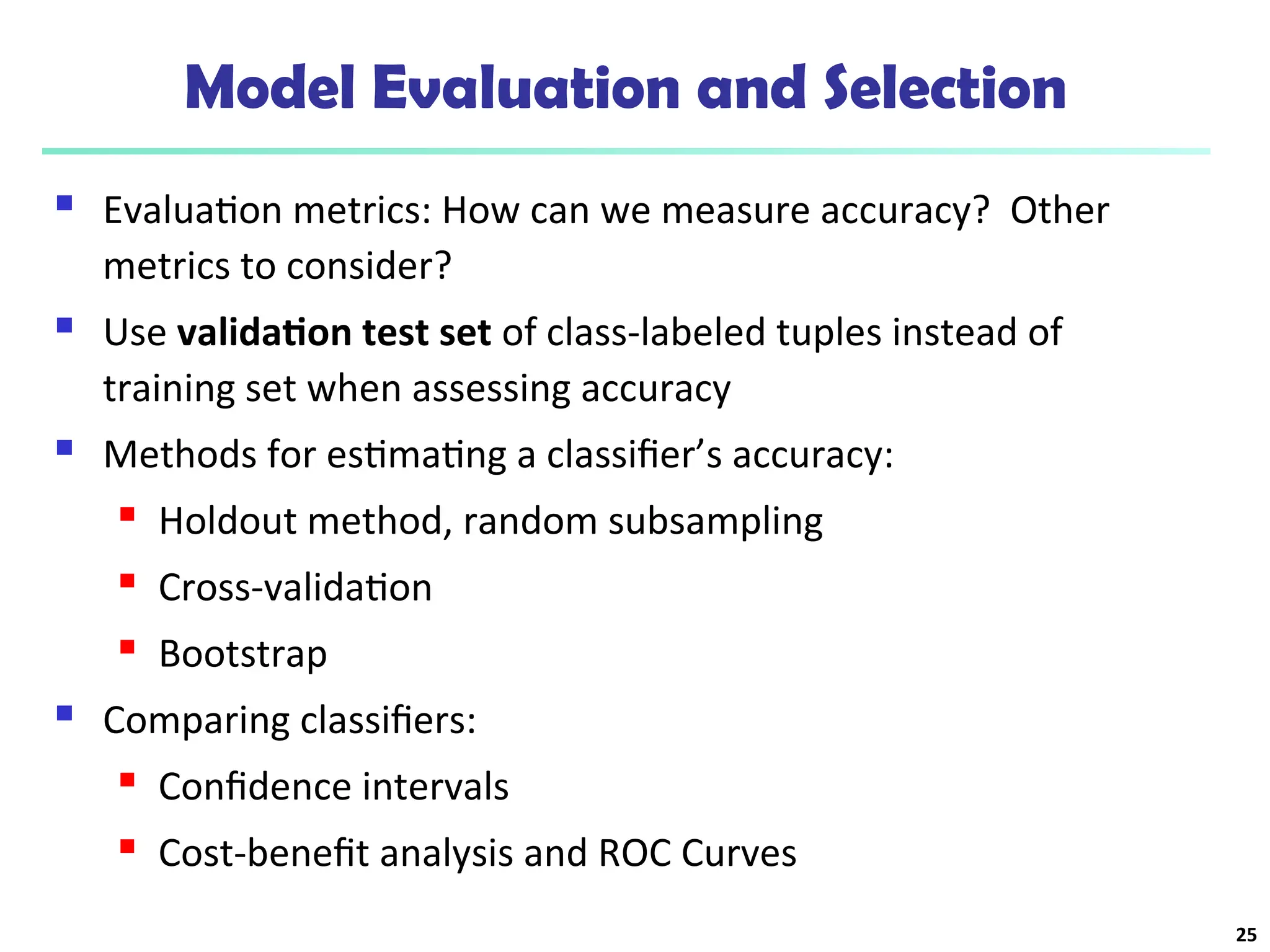
 Evaluation metrics: How can we measure accuracy? Other
metrics to consider?
 Use validation test set of class-labeled tuples instead of
training set when assessing accuracy
 Methods for estimating a classifier’s accuracy:
 Holdout method, random subsampling
 Cross-validation
 Bootstrap
 Comparing classifiers:
 Confidence intervals
 Cost-benefit analysis and ROC Curves
25

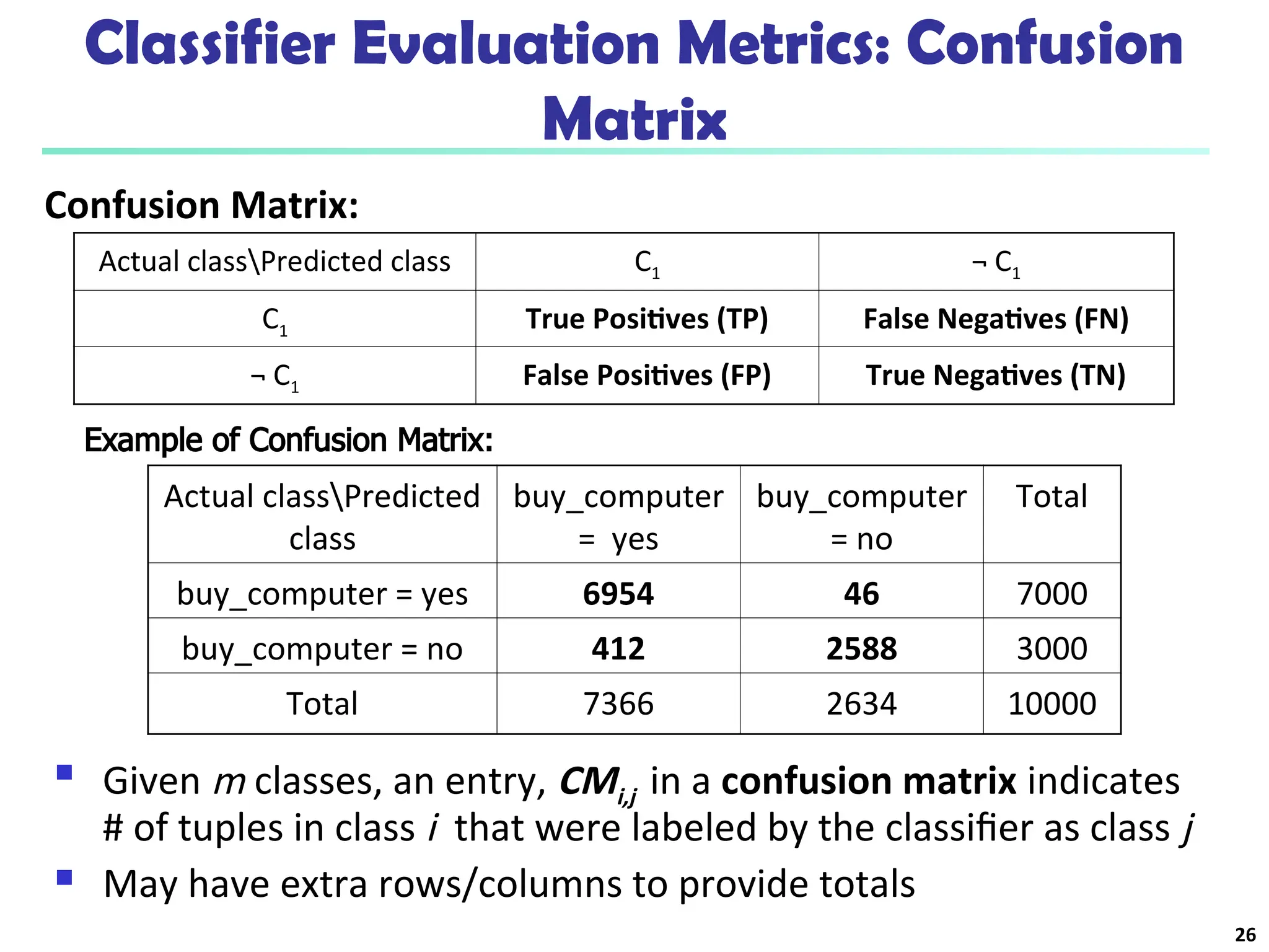
Classifier Evaluation Metrics: Confusion
Matrix
Actual classPredicted
class
buy_computer
= yes
buy_computer
= no
Total
buy_computer = yes 6954 46 7000
buy_computer = no 412 2588 3000
Total 7366 2634 10000
 Given m classes, an entry, CMi,j in a confusion matrix indicates
# of tuples in class i that were labeled by the classifier as class j
 May have extra rows/columns to provide totals
Confusion Matrix:
Actual classPredicted class C1 ¬ C1
C1 True Positives (TP) False Negatives (FN)
¬ C1 False Positives (FP) True Negatives (TN)
Example of Confusion Matrix:
26

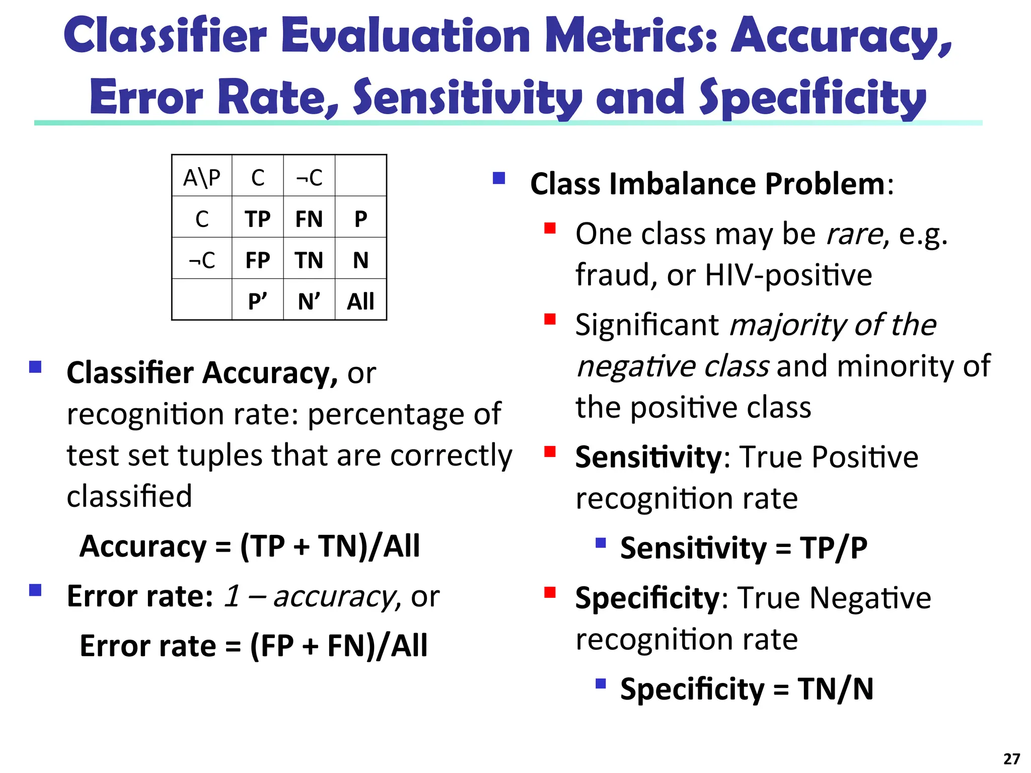
Classifier Evaluation Metrics: Accuracy,
Error Rate, Sensitivity and Specificity
 Classifier Accuracy, or
recognition rate: percentage of
test set tuples that are correctly
classified
Accuracy = (TP + TN)/All
 Error rate: 1 – accuracy, or
Error rate = (FP + FN)/All
 Class Imbalance Problem:
 One class may be rare, e.g.
fraud, or HIV-positive
 Significant majority of the
negative class and minority of
the positive class
 Sensitivity: True Positive
recognition rate

Sensitivity = TP/P
 Specificity: True Negative
recognition rate

Specificity = TN/N
AP C ¬C
C TP FN P
¬C FP TN N
P’ N’ All
27

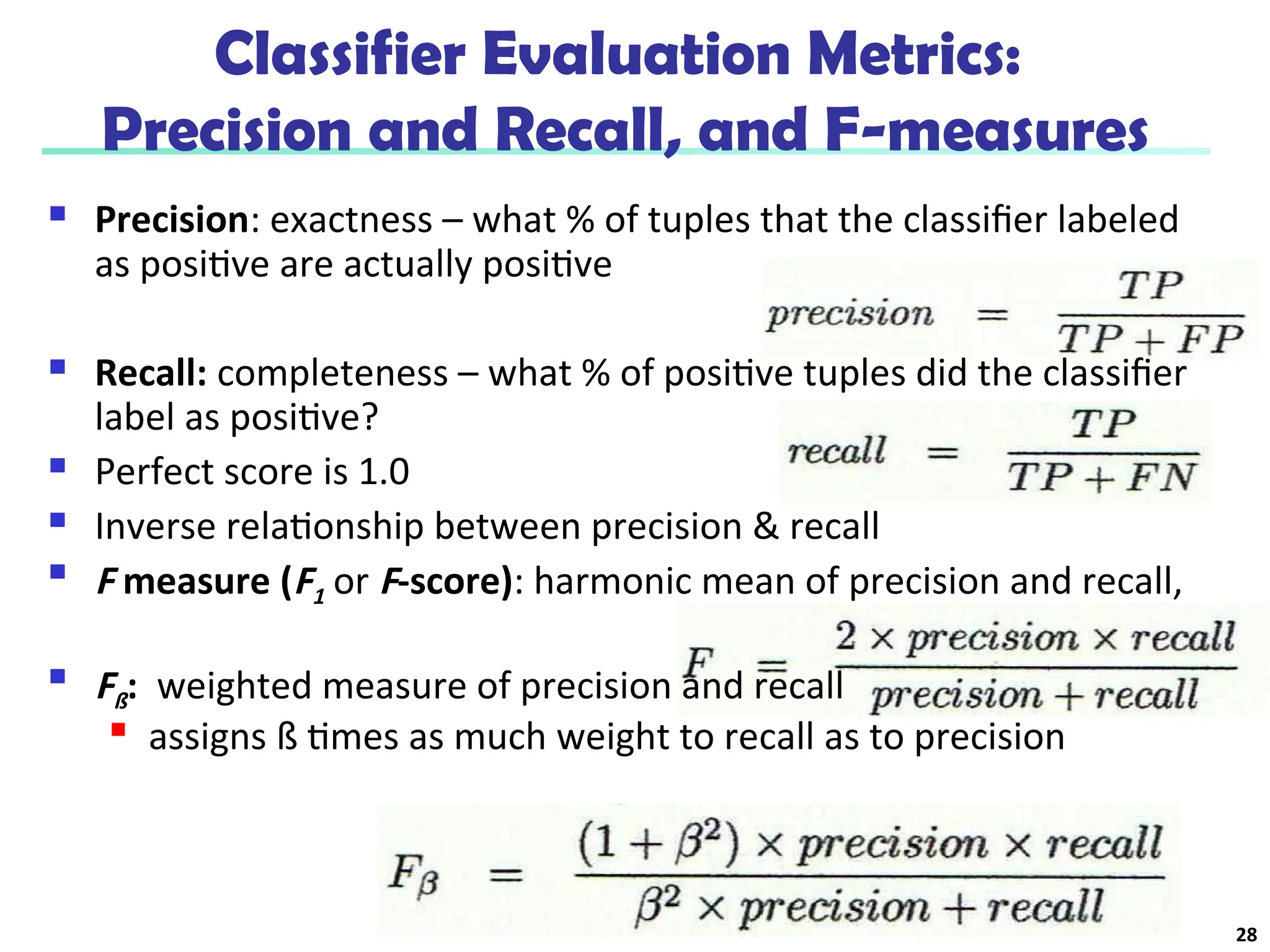
Classifier Evaluation Metrics:
Precision and Recall, and F-measures
 Precision: exactness – what % of tuples that the classifier labeled
as positive are actually positive
 Recall: completeness – what % of positive tuples did the classifier
label as positive?
 Perfect score is 1.0
 Inverse relationship between precision & recall

F measure (F1 or F-score): harmonic mean of precision and recall,

Fß: weighted measure of precision and recall

assigns ß times as much weight to recall as to precision
28

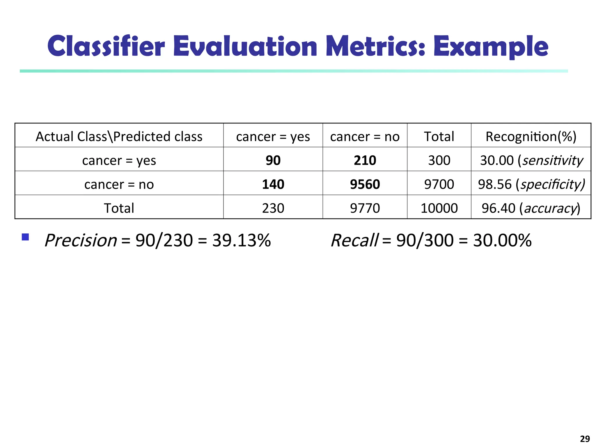
Classifier Evaluation Metrics: Example
29
 Precision = 90/230 = 39.13% Recall = 90/300 = 30.00%
Actual ClassPredicted class cancer = yes cancer = no Total Recognition(%)
cancer = yes 90 210 300 30.00 (sensitivity
cancer = no 140 9560 9700 98.56 (specificity)
Total 230 9770 10000 96.40 (accuracy)

Evaluating Classifier Accuracy:
Holdout & Cross-Validation Methods
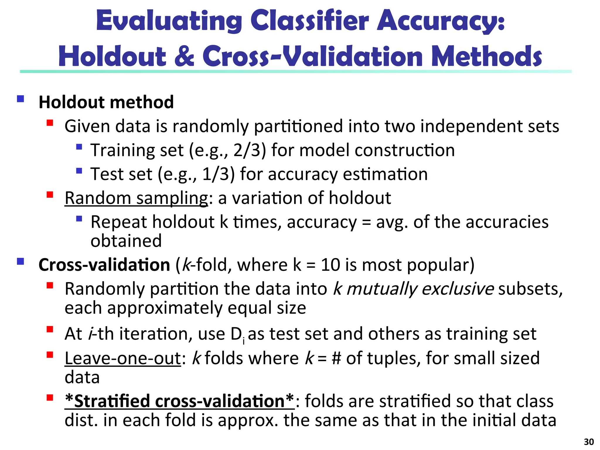
 Holdout method

Given data is randomly partitioned into two independent sets

Training set (e.g., 2/3) for model construction

Test set (e.g., 1/3) for accuracy estimation

Random sampling: a variation of holdout

Repeat holdout k times, accuracy = avg. of the accuracies
obtained
 Cross-validation (k-fold, where k = 10 is most popular)

Randomly partition the data into k mutually exclusive subsets,
each approximately equal size

At i-th iteration, use Di as test set and others as training set

Leave-one-out: k folds where k = # of tuples, for small sized
data

*Stratified cross-validation*: folds are stratified so that class
dist. in each fold is approx. the same as that in the initial data
30

Evaluating Classifier Accuracy: Bootstrap
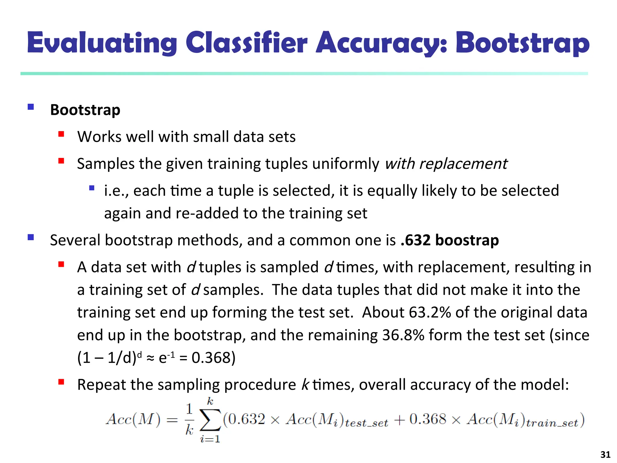
 Bootstrap
 Works well with small data sets
 Samples the given training tuples uniformly with replacement

i.e., each time a tuple is selected, it is equally likely to be selected
again and re-added to the training set
 Several bootstrap methods, and a common one is .632 boostrap
 A data set with d tuples is sampled d times, with replacement, resulting in
a training set of d samples. The data tuples that did not make it into the
training set end up forming the test set. About 63.2% of the original data
end up in the bootstrap, and the remaining 36.8% form the test set (since
(1 – 1/d)d
≈ e-1
= 0.368)
 Repeat the sampling procedure k times, overall accuracy of the model:
31

Model Selection: ROC Curves
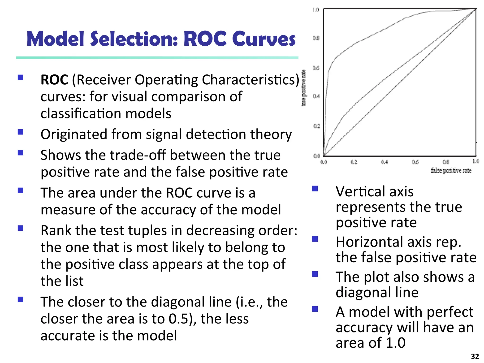
 ROC (Receiver Operating Characteristics)
curves: for visual comparison of
classification models
 Originated from signal detection theory
 Shows the trade-off between the true
positive rate and the false positive rate
 The area under the ROC curve is a
measure of the accuracy of the model
 Rank the test tuples in decreasing order:
the one that is most likely to belong to
the positive class appears at the top of
the list
 The closer to the diagonal line (i.e., the
closer the area is to 0.5), the less
accurate is the model
 Vertical axis
represents the true
positive rate
 Horizontal axis rep.
the false positive rate
 The plot also shows a
diagonal line
 A model with perfect
accuracy will have an
area of 1.0
32

Issues Affecting Model Selection
 Accuracy
 classifier accuracy: predicting class label
 Speed
 time to construct the model (training time)
 time to use the model (classification/prediction time)
 Robustness: handling noise and missing values
 Scalability: efficiency in disk-resident databases
 Interpretability
 understanding and insight provided by the model
 Other measures, e.g., goodness of rules, such as decision tree
size or compactness of classification rules
33

34
Ensemble Methods
 Summary

Ensemble Methods: Increasing the Accuracy
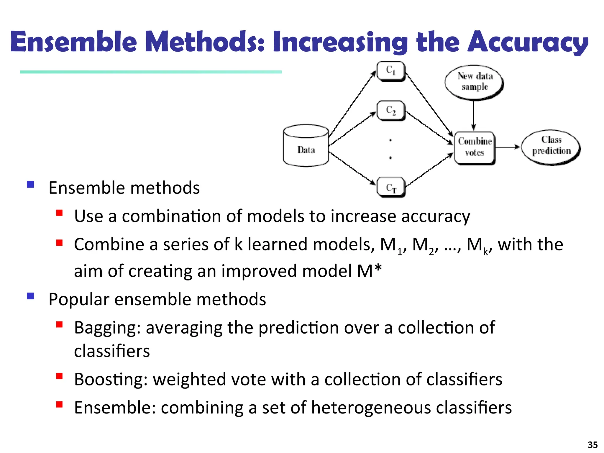
 Ensemble methods

Use a combination of models to increase accuracy
 Combine a series of k learned models, M1, M2, …, Mk, with the
aim of creating an improved model M*
 Popular ensemble methods
 Bagging: averaging the prediction over a collection of
classifiers

Boosting: weighted vote with a collection of classifiers
 Ensemble: combining a set of heterogeneous classifiers
35

Bagging: Boostrap Aggregation
 Analogy: Diagnosis based on multiple doctors’ majority vote
 Training
 Given a set D of d tuples, at each iteration i, a training set Di of d tuples is
sampled with replacement from D (i.e., bootstrap)
 A classifier model Mi is learned for each training set Di
 Classification: classify an unknown sample X
 Each classifier Mi returns its class prediction
 The bagged classifier M* counts the votes and assigns the class with the
most votes to X
 Prediction: can be applied to the prediction of continuous values by taking the
average value of each prediction for a given test tuple
 Accuracy
 Often significantly better than a single classifier derived from D
 For noise data: not considerably worse, more robust
 Proved improved accuracy in prediction
36

Boosting
 Analogy: Consult several doctors, based on a combination of
weighted diagnoses—weight assigned based on the previous
diagnosis accuracy
 How boosting works?
 Weights are assigned to each training tuple
 A series of k classifiers is iteratively learned

After a classifier Mi is learned, the weights are updated to allow
the subsequent classifier, Mi+1, to pay more attention to the
training tuples that were misclassified by Mi
 The final M* combines the votes of each individual classifier,
where the weight of each classifier's vote is a function of its
accuracy
 Boosting algorithm can be extended for numeric prediction
 Comparing with bagging: Boosting tends to have greater accuracy,
but it also risks overfitting the model to misclassified data
37

38
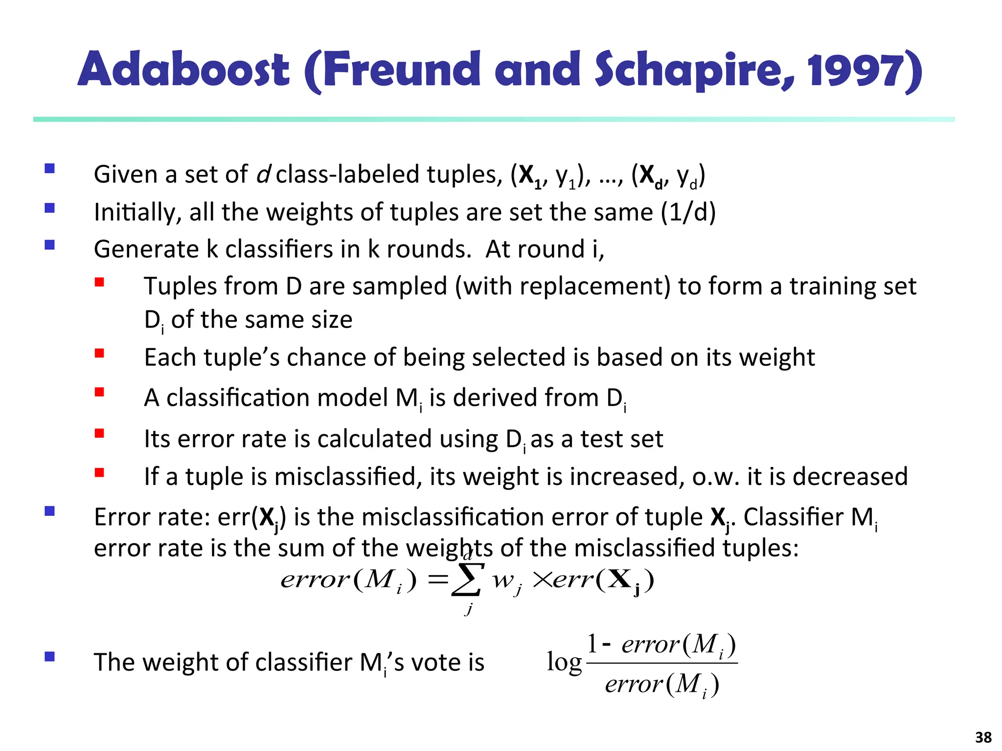
Adaboost (Freund and Schapire, 1997)
 Given a set of d class-labeled tuples, (X1, y1), …, (Xd, yd)
 Initially, all the weights of tuples are set the same (1/d)
 Generate k classifiers in k rounds. At round i,
 Tuples from D are sampled (with replacement) to form a training set
Di of the same size
 Each tuple’s chance of being selected is based on its weight

A classification model Mi is derived from Di

Its error rate is calculated using Di as a test set
 If a tuple is misclassified, its weight is increased, o.w. it is decreased
 Error rate: err(Xj) is the misclassification error of tuple Xj. Classifier Mi
error rate is the sum of the weights of the misclassified tuples:
 The weight of classifier Mi’s vote is
)
(
)
(
1
log
i
i
M
error
M
error

 

d
j
j
i err
w
M
error )
(
)
( j
X

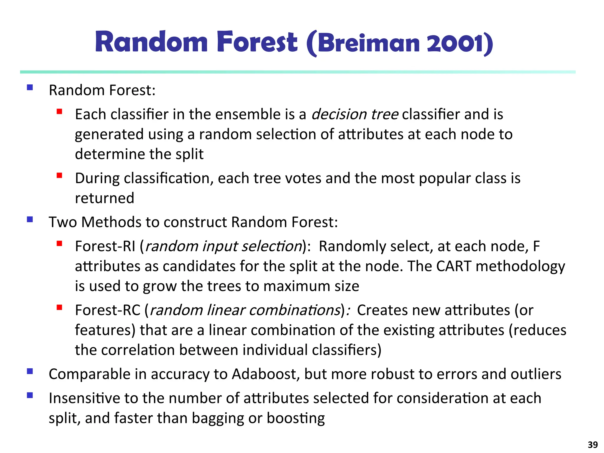
Random Forest (Breiman 2001)
 Random Forest:

Each classifier in the ensemble is a decision tree classifier and is
generated using a random selection of attributes at each node to
determine the split
 During classification, each tree votes and the most popular class is
returned
 Two Methods to construct Random Forest:
 Forest-RI (random input selection): Randomly select, at each node, F
attributes as candidates for the split at the node. The CART methodology
is used to grow the trees to maximum size
 Forest-RC (random linear combinations): Creates new attributes (or
features) that are a linear combination of the existing attributes (reduces
the correlation between individual classifiers)
 Comparable in accuracy to Adaboost, but more robust to errors and outliers
 Insensitive to the number of attributes selected for consideration at each
split, and faster than bagging or boosting
39

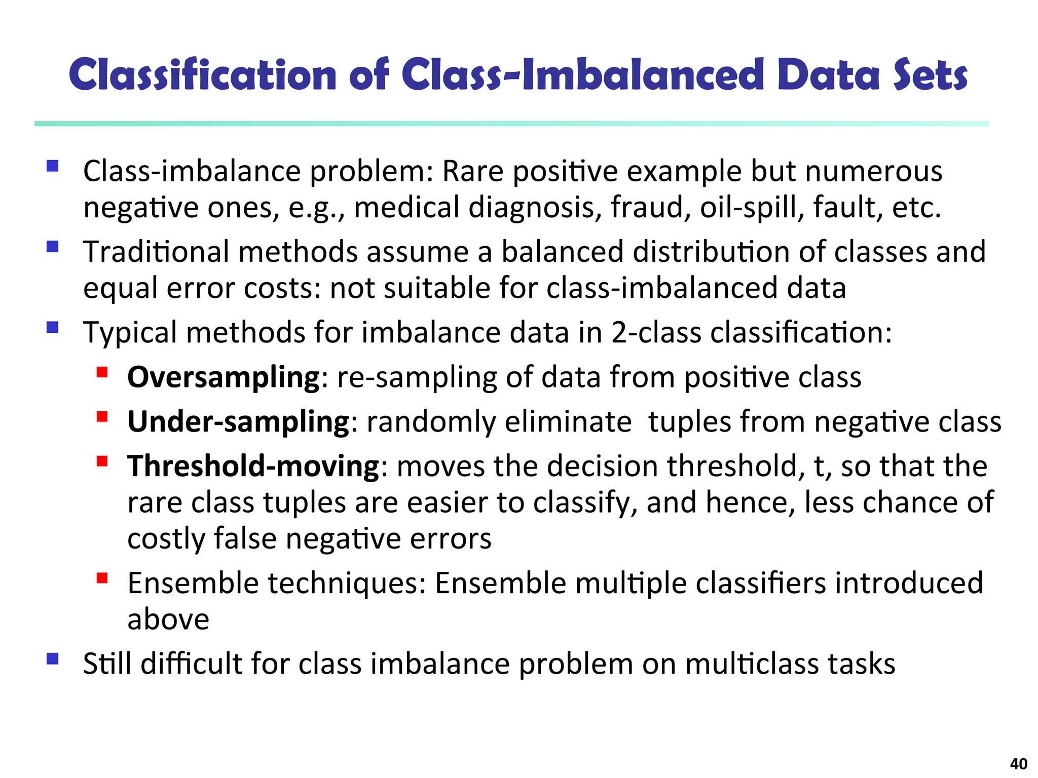
Classification of Class-Imbalanced Data Sets
 Class-imbalance problem: Rare positive example but numerous
negative ones, e.g., medical diagnosis, fraud, oil-spill, fault, etc.
 Traditional methods assume a balanced distribution of classes and
equal error costs: not suitable for class-imbalanced data
 Typical methods for imbalance data in 2-class classification:
 Oversampling: re-sampling of data from positive class
 Under-sampling: randomly eliminate tuples from negative class
 Threshold-moving: moves the decision threshold, t, so that the
rare class tuples are easier to classify, and hence, less chance of
costly false negative errors
 Ensemble techniques: Ensemble multiple classifiers introduced
above
 Still difficult for class imbalance problem on multiclass tasks
40

41
Ensemble Methods
 Summary

Summary (I)
 Classification is a form of data analysis that extracts models describing
important data classes.
 Effective and scalable methods have been developed for decision tree
induction, Naive Bayesian classification, rule-based classification, and
many other classification methods.
 Evaluation metrics include: accuracy, sensitivity, specificity, precision,
recall, F measure, and Fß measure.
 Stratified k-fold cross-validation is recommended for accuracy
estimation. Bagging and boosting can be used to increase overall
accuracy by learning and combining a series of individual models.
42

Summary (II)
 Significance tests and ROC curves are useful for model selection.
 There have been numerous comparisons of the different
classification methods; the matter remains a research topic
 No single method has been found to be superior over all others
for all data sets
 Issues such as accuracy, training time, robustness, scalability,
and interpretability must be considered and can involve trade-
offs, further complicating the quest for an overall superior
method
43

4_22865_IS465_2019_1__2_1_08ClassBasic.ppt

More Related Content

Similar to 4_22865_IS465_2019_1__2_1_08ClassBasic.ppt

More from TSANKARARAO

Recently uploaded

4_22865_IS465_2019_1__2_1_08ClassBasic.ppt

Editor's Notes