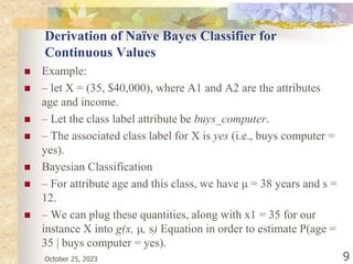
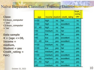
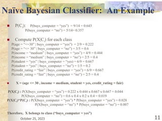
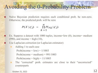
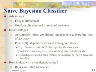
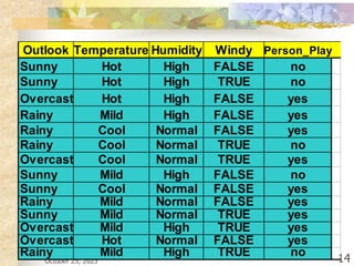
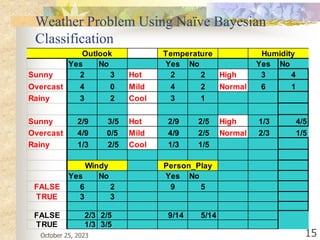
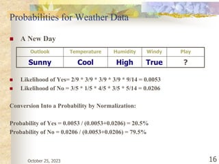
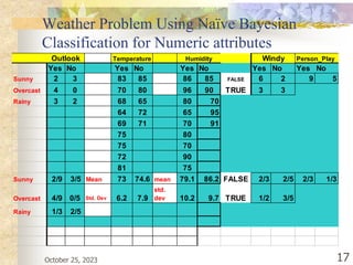
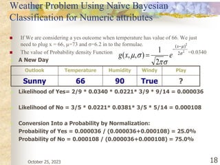
SlideShare a Scribd company logo
1 of 54
UNIT 2
Regression / Bayesian Learning / Support Vector Machine
1. Tom M. Mitchell,―Machine Learning, McGraw-Hill Education (India) Private Limited, 2013.
2. Ethem Alpaydin,―Introduction to Machine Learning (Adaptive Computation and Machine
Learning), The MIT Press 2004.
3. Stephen Marsland, ―Machine Learning: An Algorithmic Perspective, CRC Press, 2009.
4. Bishop, C., Pattern Recognition and Machine Learning. Berlin: Springer- Verlag.
1
KCS 055: Machine Learning
Dr. Neelaksh Sheel
(Associate Prof. CS & E)
CS & E Dept. M.I.T Moradabad
B.Tech CSE V sem
Recommended Books:
October 25, 2023
October 25, 2023 2
Bayesian Classification: Why?
 Bayesian classification is a probabilistic approach to learning and
inference based on a different view of what it means to learn from data, in
which probability is used to represent uncertainty about the relationship being
learnt.
 A statistical classifier: performs probabilistic prediction, i.e., predicts class
membership probabilities( that a given tuple belongs to a particular class)
 Foundation: Based on Bayes’ Theorem given by Thomas Bayes
 Class Conditional Independence : Naïve Bayesian Classifiers assume that
the effect of an attribute value on a given class is independent of the values of
the other attributes. This assumption is called class conditional independence.
 It is a classification technique based on Bayes’ Theorem with an assumption
of independence among predictors. In simple terms, a Naive Bayes classifier
assumes that the presence of a particular feature in a class is unrelated to
the presence of any other feature
 For example, a fruit may be considered to be an apple if it is red, round, and
about 3 inches in diameter. Even if these features depend on each other or
upon the existence of the other features, all of these properties independently
contribute to the probability that this fruit is an apple and that is why it is
known as ‘Naive’.
Bayesian Classification:
 Naive Bayes model is easy to build and particularly useful for very large
data sets. Along with simplicity, Naive Bayes is known to outperform even
highly sophisticated classification methods.
 Performance: A simple Bayesian classifier, naïve Bayesian classifier, has
comparable performance with decision tree and selected neural
network classifiers.
 Incremental: Each training example can incrementally
increase/decrease the probability that a hypothesis is correct — prior
knowledge can be combined with observed data
 Standard: Even when Bayesian methods are computationally intractable,
they can provide a standard of optimal decision making against which
other methods can be measured
 Bayesian Belief Network: are graphical models that allow the
representation of dependencies among subsets of attributes
October 25, 2023 3
October 25, 2023 4
Naïve Bayesian Classification
 Naïve Bayes classifier use all the attributes
 Two assumptions:
 –Attributes are equally important
 – Attributes are statistically independent
i.e., knowing the value of one attribute
says nothing about the value of another
 Equally important & independence assumptions
are never correct in real-life datasets
October 25, 2023 5
Bayesian Theorem: Basics
 Let X be a data sample (“evidence”): class label is unknown
 Let H be a hypothesis that X belongs to class C
 E.g. Our world of tuples is confined to customers described by the attributes age and
income. X is a35 year old customer with an income $40,000.
 Classification is to determine P(H|X), the probability that the hypothesis holds given
the observed data sample X. P(H|X) reflects the probability that customer X will buy a
computer given that we know the customer’s age and income.
 P(H) (prior probability), the initial probability
 E.g., X will buy computer, regardless of age, income, …
 P(X): prior probability of X. probability that sample data is observed( that a person
from our set of customers is 35 years old and earns $40,000
 P(X|H) (posteriori probability), the probability of observing the sample X, given that
the hypothesis holds
 E.g., Given that X will buy computer, the prob. that X is 31..40, medium income
October 25, 2023 6
Bayesian Theorem
 Given training data X, posteriori probability of a hypothesis H,
P(H|X), follows the Bayes theorem
 Informally, this can be written as
posteriori = likelihood x prior/evidence
 Predicts X belongs to Ci iff the probability P(Ci|X) is the
highest among all the P(Ck|X) for all the k classes
 Practical difficulty: require initial knowledge of many
probabilities, significant computational cost
)
(
)
(
)
|
(
)
|
(
X
X
X
P
H
P
H
P
H
P 
October 25, 2023 7
Towards Naïve Bayesian Classifier
 Let D be a training set of tuples and their associated class
labels, and each tuple is represented by an n-D attribute vector
X = (x1, x2, …, xn)
 Suppose there are m classes C1, C2, …, Cm.
 Classification is to derive the maximum posteriori, i.e., the
maximal P(Ci|X)
 This can be derived from Bayes’ theorem
 Since P(X) is constant for all classes, only
needs to be maximized
)
(
)
(
)
|
(
)
|
(
X
X
X
P
i
C
P
i
C
P
i
C
P 
)
(
)
|
(
)
|
(
i
C
P
i
C
P
i
C
P X
X 
October 25, 2023 8
Derivation of Naïve Bayes Classifier
 A simplified assumption: attributes are conditionally independent (i.e., no
dependence relation between attributes):
 This greatly reduces the computation cost: Only counts the class
distribution
 If Ak is categorical, P(xk|Ci) is the # of tuples in Ci having value xk for Ak
divided by |Ci, D| (# of tuples of Ci in D)
 If Ak is continous-valued, P(xk|Ci) is usually computed based on Gaussian
distribution with a mean μ and standard deviation σ
and P(xk|Ci) is
)
|
(
...
)
|
(
)
|
(
1
)
|
(
)
|
(
2
1
Ci
x
P
Ci
x
P
Ci
x
P
n
k
Ci
x
P
Ci
P
n
k







X
2
2
2
)
(
2
1
)
,
,
( 








x
e
x
g
)
,
,
(
)
|
( i
i C
C
k
x
g
Ci
P 


X
October 25, 2023 9
Derivation of Naïve Bayes Classifier for
Continuous Values
 Example:
 – let X = (35, $40,000), where A1 and A2 are the attributes
age and income.
 – Let the class label attribute be buys_computer.
 – The associated class label for X is yes (i.e., buys computer =
yes).
 Bayesian Classification
 – For attribute age and this class, we have μ = 38 years and s =
12.
 – We can plug these quantities, along with x1 = 35 for our
instance X into g(x, μ, s) Equation in order to estimate P(age =
35 | buys computer = yes).
October 25, 2023 10
Naïve Bayesian Classifier: Training Dataset
Class:
C1:buys_computer
= ‘yes’
C2:buys_computer
= ‘no’
Data sample
X = (age <=30,
Income =
medium,
Student = yes
Credit_rating =
Fair)
age income student credit_rating
buys_
comp
uter
<=30 high no fair no
<=30 high no excellent no
31…40 high no fair yes
>40 medium no fair yes
>40 low yes fair yes
>40 low yes excellent no
31…40 low yes excellent yes
<=30 medium no fair no
<=30 low yes fair yes
>40 medium yes fair yes
<=30 medium yes excellent yes
31…40 medium no excellent yes
31…40 high yes fair yes
>40 medium no excellent no
October 25, 2023 11
Naïve Bayesian Classifier: An Example
 P(Ci): P(buys_computer = “yes”) = 9/14 = 0.643
P(buys_computer = “no”) = 5/14= 0.357
 Compute P(X|Ci) for each class
P(age = “<=30” | buys_computer = “yes”) = 2/9 = 0.222
P(age = “<= 30” | buys_computer = “no”) = 3/5 = 0.6
P(income = “medium” | buys_computer = “yes”) = 4/9 = 0.444
P(income = “medium” | buys_computer = “no”) = 2/5 = 0.4
P(student = “yes” | buys_computer = “yes) = 6/9 = 0.667
P(student = “yes” | buys_computer = “no”) = 1/5 = 0.2
P(credit_rating = “fair” | buys_computer = “yes”) = 6/9 = 0.667
P(credit_rating = “fair” | buys_computer = “no”) = 2/5 = 0.4
 X = (age <= 30 , income = medium, student = yes, credit_rating = fair)
P(X|Ci) : P(X|buys_computer = “yes”) = 0.222 x 0.444 x 0.667 x 0.667 = 0.044
P(X|buys_computer = “no”) = 0.6 x 0.4 x 0.2 x 0.4 = 0.019
P(X|Ci)*P(Ci) : P(X|buys_computer = “yes”) * P(buys_computer = “yes”) = 0.028
P(X|buys_computer = “no”) * P(buys_computer = “no”) = 0.007
Therefore, X belongs to class (“buys_computer = yes”)
October 25, 2023 12
Avoiding the 0-Probability Problem
 Naïve Bayesian prediction requires each conditional prob. be non-zero.
Otherwise, the predicted prob. will be zero
 Ex. Suppose a dataset with 1000 tuples, income=low (0), income= medium
(990), and income = high (10),
 Use Laplacian correction (or Laplacian estimator)
 Adding 1 to each case
Prob(income = low) = 1/1003
Prob(income = medium) = 991/1003
Prob(income = high) = 11/1003
 The “corrected” prob. estimates are close to their “uncorrected”
counterparts



n
k
Ci
xk
P
Ci
X
P
1
)
|
(
)
|
(
October 25, 2023 13
Naïve Bayesian Classifier
 Advantages
 Easy to implement
 Good results obtained in most of the cases
 Disadvantages
 Assumption: class conditional independence, therefore loss
of accuracy
 Practically, dependencies exist among variables
 E.g., hospitals: patients: Profile: age, family history, etc.
Symptoms: fever, cough etc., Disease: lung cancer, diabetes, etc.
 Dependencies among these cannot be modeled by Naïve Bayesian
Classifier
 How to deal with these dependencies?
 Bayesian Belief Networks
October 25, 2023 14
Weather Problem Using Naïve Bayesian
Classification
Outlook Temperature Humidity Windy Person_Play
Sunny Hot High FALSE no
Sunny Hot High TRUE no
Overcast Hot High FALSE yes
Rainy Mild High FALSE yes
Rainy Cool Normal FALSE yes
Rainy Cool Normal TRUE no
Overcast Cool Normal TRUE yes
Sunny Mild High FALSE no
Sunny Cool Normal FALSE yes
Rainy Mild Normal FALSE yes
Sunny Mild Normal TRUE yes
Overcast Mild High TRUE yes
Overcast Hot Normal FALSE yes
Rainy Mild High TRUE no
October 25, 2023 15
Weather Problem Using Naïve Bayesian
Classification
Yes No Yes No Yes No
Sunny 2 3 Hot 2 2 High 3 4
Overcast 4 0 Mild 4 2 Normal 6 1
Rainy 3 2 Cool 3 1
Sunny 2/9 3/5 Hot 2/9 2/5 High 1/3 4/5
Overcast 4/9 0/5 Mild 4/9 2/5 Normal 2/3 1/5
Rainy 1/3 2/5 Cool 1/3 1/5
Yes No Yes No
FALSE 6 2 9 5
TRUE 3 3
FALSE 2/3 2/5 9/14 5/14
TRUE 1/3 3/5
Humidity
Windy Person_Play
Outlook Temperature
October 25, 2023 16
Probabilities for Weather Data
 A New Day
 Likelihood of Yes= 2/9 * 3/9 * 3/9 * 3/9 * 9/14 = 0.0053
 Likelihood of No = 3/5 * 1/5 * 4/5 * 3/5 * 5/14 = 0.0206
Conversion Into a Probability by Normalization:
Probability of Yes = 0.0053 / (0.0053+0.0206) = 20.5%
Probability of No = 0.0206 / (0.0053+0.0206) = 79.5%
Outlook Temperature Humidity Windy Play
Sunny Cool High True ?
October 25, 2023 17
Weather Problem Using Naïve Bayesian
Classification for Numeric attributes
Person_Play
Yes No Yes No Yes No Yes No Yes No
Sunny 2 3 83 85 86 85 FALSE 6 2 9 5
Overcast 4 0 70 80 96 90 TRUE 3 3
Rainy 3 2 68 65 80 70
64 72 65 95
69 71 70 91
75 80
75 70
72 90
81 75
Sunny 2/9 3/5 Mean 73 74.6 mean 79.1 86.2 FALSE 2/3 2/5 2/3 1/3
Overcast 4/9 0/5 Std. Dev 6.2 7.9
std.
dev 10.2 9.7 TRUE 1/2 3/5
Rainy 1/3 2/5
Humidity Windy
Outlook Temperature
October 25, 2023 18
Weather Problem Using Naïve Bayesian
Classification for Numeric attributes
 If We are considering a yes outcome when temperature has value of 66. We just
need to plug x = 66, µ=73 and σ=6.2 in to the formulae.
 The value of Probability density Function =0.0340
2
2
2
)
(
2
1
)
,
,
( 








x
e
x
g
 A New Day
 Likelihood of Yes= 2/9 * 0.0340 * 0.0221* 3/9 * 9/14 = 0.000036
 Likelihood of No = 3/5 * 0.0221* 0.0381* 3/5 * 5/14 = 0.000108
 Conversion Into a Probability by Normalization:
Probability of Yes = 0.000036 / (0.000036+0.000108) = 25.0%
Probability of No = 0.000108 / (0.000036+0.000108) = 75.0%
Outlook Temperature Humidity Windy Play
Sunny 66 90 True ?
October 25, 2023 19
Bayesian Belief Networks
 A Bayesian network (or a belief network) is a probabilistic graphical model that represents a
set of variables and their probabilistic independencies. For example, a Bayesian network could
represent the probabilistic relationships between diseases and symptoms. Given symptoms, the
network can be used to compute the probabilities of the presence of various diseases. Bayesian
belief network allows a subset of the variables conditionally independent
 Bayesian Belief Networks is defined by two components
a) A Directed acyclic graph b) A set of conditional Probability Tables
 A graphical model of causal relationships
 Represents dependency among the variables
 Gives a specification of joint probability distribution
X Y
Z
P
 Nodes: random variables
 Links: dependency
 X & Y are the parents of Z, & Y is the parent of P
 No dependency between Z and P
 Has no loops or cycles
Inference with more complex dependencies
• How do we represent (model) more complex probabilistic relationships?
• How do we use these models to draw inferences?
Probabilistic reasoning
• Let us take an example. Suppose I go to my house and see that the door is
open.
- What’s the cause? Is it a burglar? Should we go in? Call the police?
- Then again, it could just be my wife. Maybe she came home early.
• How should we represent these relationships?
Belief networks
• In Belief networks, causal relationships are represented in directed acyclic
graphs.
• Arrows indicate causal relationships between the nodes.
October 25, 2023 20
Wife Burglar
Open Door
Types of Probabilistic Relationships
 How do we represent these relationships?
 Direct Cause Indirect Cause Common Cause Common Effect
 P(B|A) P(B|A) P(B|A) P(C|A,B)
P(C|B) P(C|A)
C is independent Are B and C Are A and B
of A given B independent? independent
October 25, 2023 21
A
B
A A A
B
B
B
C
C
C
Belief Networks
 • In Belief networks, causal relationships are represented in directed
acyclic graphs. Arrows indicate causal relationships between the nodes.
 Explaining away
•Suppose we notice that the car is in the garage.
• Now we infer that it’s probably my wife, and not a burglar.
• This fact “explains away” the hypothesis of a burglar.
October 25, 2023 22
Wife Burglar
Open Door
How can we determine what is
happening before we go in?
We need more
information. What
else can we
observe?
Wife Burglar
Open Door
Car in Garage
Note that there is no
direct causal link
between “burglar”
and “car in garage”.
Yet, seeing the car
changes our beliefs
about the burglar.
Belief Networks
 We could also notice the door was damaged, in which case we reach the
opposite conclusion.
 Defining the belief network
 • Each link in the graph represents a conditional relationship between nodes.
 • To compute the inference, we must specify the conditional probabilities.
October 25, 2023 23
Let’s start by
writing down
the conditional
probabilities
Wife Burglar
Open
Door
Car in
Garage
Damaged
Door
How do we make
this inference
process more
precise?
October 25, 2023 24
Bayesian Belief Network: An Example
Family
History
LungCancer
PositiveXRay
Smoker
Emphysema
Dyspnea
LC
~LC
(FH, S) (FH, ~S) (~FH, S) (~FH, ~S)
0.8
0.2
0.5
0.5
0.7
0.3
0.1
0.9
Bayesian Belief Networks
The conditional probability table
(CPT) for variable LungCancer:



n
i
Y
Parents i
xi
P
x
x
P n
1
))
(
|
(
)
,...,
( 1
CPT shows the conditional probability
for each possible combination of its
parents
Derivation of the probability of a particular
combination of values of X, from CPT:
October 25, 2023 25
Training Bayesian Networks
 Several scenarios:
 Given both the network structure and all
variables observable: learn only the CPTs
 Network structure known, some hidden variables:
gradient descent (greedy hill-climbing) method,
analogous to neural network learning
 Network structure unknown, all variables
observable: search through the model space to
reconstruct network topology
 Unknown structure, all hidden variables: No
good algorithms known for this purpose
Bayesian Belief Network: An Example
October 25, 2023 26
Bayesian Belief Network: An Example
October 25, 2023 27
Bayesian Belief Network: An Example
October 25, 2023 28
Expectation–Maximization (EM) algorithm
In statistics, an expectation–maximization (EM) algorithm is
an iterative method to find (local) maximum
likelihood or maximum a posteriori (MAP) estimates
of parameters in statistical models, where the model depends on
unobserved latent variables. The EM iteration alternates between
performing an expectation (E) step, which creates a function for
the expectation of the log-likelihood evaluated using the current
estimate for the parameters, and a maximization (M) step, which
computes parameters maximizing the expected log-likelihood
found on the E step. These parameter-estimates are then used to
determine the distribution of the latent variables in the next E
step.
October 25, 2023 29
October 25, 2023 30
The EM algorithm is considered a latent variable model to find the
local maximum likelihood parameters of a statistical model,
proposed by Arthur Dempster, Nan Laird, and Donald Rubin in
1977.
The EM (Expectation-Maximization) algorithm is one of the most
commonly used terms in machine learning to obtain maximum
likelihood estimates of variables that are sometimes observable and
sometimes not. However, it is also applicable to unobserved data or
sometimes called latent. It has various real-world applications in
statistics, including obtaining the mode of the posterior marginal
distribution of parameters in machine learning and data
mining applications.
What is an EM algorithm?
 The Expectation-Maximization (EM) algorithm is defined as the
combination of various unsupervised machine learning
algorithms, which is used to determine the local maximum
likelihood estimates (MLE) or maximum a posteriori estimates
(MAP) for unobservable variables in statistical models. Further, it
is a technique to find maximum likelihood estimation when the
latent variables are present. It is also referred to as the latent
variable model.
 A latent variable model consists of both observable and
unobservable variables where observable can be predicted while
unobserved are inferred from the observed variable. These
unobservable variables are known as latent variables.
October 25, 2023 31
 Expectation step (E - step): It involves the estimation (guess)
of all missing values in the dataset so that after completing this
step, there should not be any missing value.
 Maximization step (M - step): This step involves the use of
estimated data in the E-step and updating the parameters.
 Repeat E-step and M-step until the convergence of the values
occurs.
October 25, 2023 32
Convergence in the EM algorithm?
Convergence is defined as the specific situation
in probability based on intuition, e.g., if there are
two random variables that have very less
difference in their probability, then they are known
as converged. In other words, whenever the values
of given variables are matched with each other, it
is called convergence.
October 25, 2023 33
Steps in EM Algorithm
October 25, 2023 34
The EM algorithm is completed mainly in 4 steps, which include
Initialization Step, Expectation Step, Maximization Step, and
convergence Step.
 1st Step: The very first step is to initialize the parameter values.
Further, the system is provided with incomplete observed data with
the assumption that data is obtained from a specific model.
 2nd Step: This step is known as Expectation or E-Step, which is used
to estimate or guess the values of the missing or incomplete data using
the observed data. Further, E-step primarily updates the variables.
 3rd Step: This step is known as Maximization or M-step, where we
use complete data obtained from the 2nd step to update the parameter
values. Further, M-step primarily updates the hypothesis.
 4th step: The last step is to check if the values of latent variables are
converging or not. If it gets "yes", then stop the process; else, repeat
the process from step 2 until the convergence occurs.
October 25, 2023 35
Regression Analysis in Machine learning
Regression analysis is a statistical method to model the
relationship between a dependent (target) and independent
(predictor) variables with one or more independent
variables. More specifically, Regression analysis helps us
to understand how the value of the dependent variable is
changing corresponding to an independent variable when
other independent variables are held fixed. It predicts
continuous/real values such as temperature, age, salary,
price, etc.
October 25, 2023 36
Example: Suppose there is a marketing company A, who does
various advertisement every year and get sales on that. The below list
shows the advertisement made by the company in the last 5 years and
the corresponding sales:
October 25, 2023 37
Now, the company wants to do
the advertisement of $200 in the
year 2019 and wants to know
the prediction about the sales
for this year.
So to solve such type of
prediction problems in machine
learning, we need regression
analysis.
Regression is a supervised learning technique which helps in finding
the correlation between variables and enables us to predict the
continuous output variable based on the one or more predictor
variables. It is mainly used for prediction, forecasting, time series
modeling, and determining the causal-effect relationship
between variables.
Regression shows a line or curve that passes through all the
datapoints on target-predictor graph in such a way that the
vertical distance between the datapoints and the regression line
is minimum. The distance between datapoints and line tells whether
a model has captured a strong relationship or not.
Examples of regression can be as:
 Prediction of rain using temperature and other factors
 Determining Market trends
 Prediction of road accidents due to rash driving.
October 25, 2023 38
Terminologies Related to the Regression Analysis:
 Dependent Variable: The main factor in Regression analysis which we want to
predict or understand is called the dependent variable. It is also called target
variable.
 Independent Variable: The factors which affect the dependent variables or
which are used to predict the values of the dependent variables are called
independent variable, also called as a predictor.
 Outliers: Outlier is an observation which contains either very low value or very
high value in comparison to other observed values. An outlier may hamper the
result, so it should be avoided.
 Multicollinearity: If the independent variables are highly correlated with each
other than other variables, then such condition is called Multicollinearity. It
should not be present in the dataset, because it creates problem while ranking the
most affecting variable.
 Underfitting and Overfitting: If our algorithm works well with the training
dataset but not well with test dataset, then such problem is called Overfitting.
And if our algorithm does not perform well even with training dataset, then such
problem is called underfitting.
October 25, 2023 39
Why do we use Regression Analysis?
 Regression estimates the relationship between
the target and the independent variable.
 It is used to find the trends in data.
 It helps to predict real/continuous values.
 By performing the regression, we can
confidently determine the most important
factor, the least important factor, and how
each factor is affecting the other factors.
October 25, 2023 40
October 25, 2023 41
Linear Regression:
 Linear regression is a statistical regression method which is used for
predictive analysis.
 It is one of the very simple and easy algorithms which works on
regression and shows the relationship between the continuous variables.
 It is used for solving the regression problem in machine learning.
 Linear regression shows the linear relationship between the independent
variable (X-axis) and the dependent variable (Y-axis), hence called linear
regression.
 If there is only one input variable (x), then such linear regression is
called simple linear regression. And if there is more than one input
variable, then such linear regression is called multiple linear regression.
 The relationship between variables in the linear regression model can be
explained using the below image. Here we are predicting the salary of an
employee on the basis of the year of experience.
October 25, 2023 42
October 25, 2023 43
Mathematical equation for Linear regression
Y= aX+b
Here,
Y = dependent variables (target variables),
X= Independent variables (predictor variables),
a and b are the linear coefficients
Applications:
•Analyzing trends and sales
estimates
•Salary forecasting
•Real estate prediction
•Arriving at Estimate time arrival
(ETA) in traffic.
Logistic Regression:
 Logistic regression is another supervised learning algorithm which is used
to solve the classification problems. In classification problems, we have
dependent variables in a binary or discrete format such as 0 or 1.
 Logistic regression algorithm works with the categorical variable such as 0
or 1, Yes or No, True or False, Spam or not spam, etc.
 It is a predictive analysis algorithm which works on the concept of
probability.
 Logistic regression is a type of regression, but it is different from the linear
regression algorithm in the term how they are used.
 Logistic regression uses sigmoid function or logistic function which is a
complex cost function. This sigmoid function is used to model the data in
logistic regression. The function can be represented as:
Where: f(x)= Output between the 0 and 1 value.
x= input to the function
e= base of natural logarithm.
October 25, 2023 44
When we provide the input values (data) to the function, it gives
the S-curve as follows:
October 25, 2023 45
•It uses the concept of threshold levels, values above the threshold level are
rounded up to 1, and values below the threshold level are rounded up to 0.
Types of logistic regression:
•Binary (0/1, pass/fail)
•Multi (cats, dogs, lions)
•Ordinal (low, medium, high)
Support Vector Machine ( SVM
 Support Vector Machine or SVM is one of the most popular Supervised
Learning algorithms, which is used for Classification as well as Regression
problems. However, primarily, it is used for Classification problems in
Machine Learning.
 The goal of the SVM algorithm is to create the best line or decision boundary
that can segregate n-dimensional space into classes so that we can easily put
the new data point in the correct category in the future. This best decision
boundary is called a hyperplane.
 SVM chooses the extreme points/vectors that help in creating the hyperplane.
These extreme cases are called as support vectors, and hence algorithm is
termed as Support Vector Machine. Consider the below diagram in which
there are two different categories that are classified using a decision boundary
or hyperplane:
October 25, 2023 46
 Applications- SVM
algorithm can be used
for Face detection,
image classification,
text categorization, and
in bioinformatics
(Protein classification,
Cancer
classification)etc.
October 25, 2023 47
Types of SVM
 Linear SVM: Linear SVM is used for linearly
separable data, which means if a dataset can be
classified into two classes by using a single straight
line, then such data is termed as linearly separable
data, and classifier is used called as Linear SVM
classifier.
 Non-linear SVM: Non-Linear SVM is used for non-
linearly separated data, which means if a dataset
cannot be classified by using a straight line, then such
data is termed as non-linear data and classifier used is
called as Non-linear SVM classifier
October 25, 2023 48
Hyperplane and Support Vectors in the SVM
algorithm:
Hyperplanes are decision boundaries that help classify the data
points. Data points falling on either side of the hyperplane can be
attributed to different classes. It is a subspace whose dimension is
one less than that of its ambient space. If a space is 3-dimensional
then its hyperplanes are the 2-dimensional planes, while if
the space is 2-dimensional, its hyperplanes are the 1-dimensional
lines. There can be multiple lines/decision boundaries to segregate
the classes in n-dimensional space, but we need to find out the best
decision boundary that helps to classify the data points. This best
boundary is known as the hyperplane of SVM.
October 25, 2023 49
The dimensions of the hyperplane depend on the
features present in the dataset, which means if there
are 2 features (as shown in image), then hyperplane
will be a straight line. And if there are 3 features, then
hyperplane will be a 2-dimension plane and so on
We always create a hyperplane that has a maximum margin, which
means the maximum distance between the data points. So, key idea
behind the SVM is to maximize the margin.
Support Vectors:
The data points or vectors that are the closest to the hyperplane and
which affect the position of the hyperplane are termed as Support
Vector. Since these vectors support the hyperplane, hence called a
Support vector.
October 25, 2023 50
Issues in SVM- SVM algorithm is not suitable for large data
sets. SVM does not perform very well when the data set has more
noise i.e. target classes are overlapping. In cases where the number
of features for each data point exceeds the number of
training data samples, the SVM will underperform.
Support Vector Machine for Multi-Class Problems
To perform SVM on multi-class problems, we can create a binary
classifier for each class of the data. The two results of each
classifier will be :
 The data point belongs to that class OR
 The data point does not belong to that class.
October 25, 2023 51
SVM for complex (Non Linearly Separable)
 SVM works very well without any modifications for linearly
separable data. Linearly Separable Data is any data that can be
plotted in a graph and can be separated into classes using a
straight line
October 25, 2023 52
We use Kernelized SVM for non-linearly separable
data. Say, we have some non-linearly separable
data in one dimension. We can transform this data into
two-dimensions and the data will become linearly
separable in two dimensions. This is done by mapping
each 1-D data point to a corresponding 2-D ordered pair.
So for any non-linearly separable data in any dimension,
we can just map the data to a higher dimension and then
make it linearly separable. This is a very powerful and
general transformation
October 25, 2023 53
Kernel in SVM:
1. Linear Kernel is used when the data is Linearly separable,
that is, it can be separated using a single Line. It is one of the most
common kernels to be used. It is mostly used when there are a
Large number of Features in a particular Data Set. One of the
examples where there are a lot of features, is Text Classification, as
each alphabet is a new feature. So we mostly use Linear Kernel in
Text Classification.
2. Polynomial Kernel : It is popular in image processing equation is:
k(Xi,Xj)=(Xi*Xj+1)d ( Where d is the degree of polynomial)
3. Gaussian Kernel:
It is a general-purpose kernel; used when there is no prior knowledge about the
data. Equation is:
||X1 — X2 || = Euclidean distance between X1 & X2
October 25, 2023 54

More Related Content

Similar to Unit-2.ppt

CS583-supervised-learning.ppt
CS583-supervised-learning.pptCS583-supervised-learning.ppt
CS583-supervised-learning.pptssuser764276
 
CS583-supervised-learning.ppt
CS583-supervised-learning.pptCS583-supervised-learning.ppt
CS583-supervised-learning.pptCaesarMaulana2
 
CS583-supervised-learning (1).ppt
CS583-supervised-learning (1).pptCS583-supervised-learning (1).ppt
CS583-supervised-learning (1).pptssuserec53e73
 
CS583-supervised-learning.ppt
CS583-supervised-learning.pptCS583-supervised-learning.ppt
CS583-supervised-learning.pptnaima768128
 
CS583-supervised-learning (3).ppt
CS583-supervised-learning (3).pptCS583-supervised-learning (3).ppt
CS583-supervised-learning (3).pptsagfjhsgh
 
CS583-supervised-learning.ppt CS583-supervised-learning
CS583-supervised-learning.ppt CS583-supervised-learningCS583-supervised-learning.ppt CS583-supervised-learning
CS583-supervised-learning.ppt CS583-supervised-learningcmpt cmpt
 
Naïve Bayes Machine Learning Classification with R Programming: A case study ...
Naïve Bayes Machine Learning Classification with R Programming: A case study ...Naïve Bayes Machine Learning Classification with R Programming: A case study ...
Naïve Bayes Machine Learning Classification with R Programming: A case study ...SubmissionResearchpa
 
Introduction to Machine Learning Aristotelis Tsirigos
Introduction to Machine Learning Aristotelis Tsirigos Introduction to Machine Learning Aristotelis Tsirigos
Introduction to Machine Learning Aristotelis Tsirigos butest
 
Data classification sammer
Data classification sammer Data classification sammer
Data classification sammer Sammer Qader
 
Data.Mining.C.6(II).classification and prediction
Data.Mining.C.6(II).classification and predictionData.Mining.C.6(II).classification and prediction
Data.Mining.C.6(II).classification and predictionMargaret Wang
 
Computational Biology, Part 4 Protein Coding Regions
Computational Biology, Part 4 Protein Coding RegionsComputational Biology, Part 4 Protein Coding Regions
Computational Biology, Part 4 Protein Coding Regionsbutest
 
3_learning.ppt
3_learning.ppt3_learning.ppt
3_learning.pptbutest
 
Bayes Classification
Bayes ClassificationBayes Classification
Bayes Classificationsathish sak
 
Boosting dl concept learners
Boosting dl concept learners Boosting dl concept learners
Boosting dl concept learners Giuseppe Rizzo
 
Intro to Model Selection
Intro to Model SelectionIntro to Model Selection
Intro to Model Selectionchenhm
 

Similar to Unit-2.ppt (20)

18 ijcse-01232
18 ijcse-0123218 ijcse-01232
18 ijcse-01232
 
CS583-supervised-learning.ppt
CS583-supervised-learning.pptCS583-supervised-learning.ppt
CS583-supervised-learning.ppt
 
CS583-supervised-learning.ppt
CS583-supervised-learning.pptCS583-supervised-learning.ppt
CS583-supervised-learning.ppt
 
CS583-supervised-learning (1).ppt
CS583-supervised-learning (1).pptCS583-supervised-learning (1).ppt
CS583-supervised-learning (1).ppt
 
CS583-supervised-learning.ppt
CS583-supervised-learning.pptCS583-supervised-learning.ppt
CS583-supervised-learning.ppt
 
CS583-supervised-learning (3).ppt
CS583-supervised-learning (3).pptCS583-supervised-learning (3).ppt
CS583-supervised-learning (3).ppt
 
CS583-supervised-learning.ppt CS583-supervised-learning
CS583-supervised-learning.ppt CS583-supervised-learningCS583-supervised-learning.ppt CS583-supervised-learning
CS583-supervised-learning.ppt CS583-supervised-learning
 
CS583-supervised-learning.ppt
CS583-supervised-learning.pptCS583-supervised-learning.ppt
CS583-supervised-learning.ppt
 
My7class
My7classMy7class
My7class
 
Naïve Bayes Machine Learning Classification with R Programming: A case study ...
Naïve Bayes Machine Learning Classification with R Programming: A case study ...Naïve Bayes Machine Learning Classification with R Programming: A case study ...
Naïve Bayes Machine Learning Classification with R Programming: A case study ...
 
Introduction to Machine Learning Aristotelis Tsirigos
Introduction to Machine Learning Aristotelis Tsirigos Introduction to Machine Learning Aristotelis Tsirigos
Introduction to Machine Learning Aristotelis Tsirigos
 
Data classification sammer
Data classification sammer Data classification sammer
Data classification sammer
 
Naive Bayes Presentation
Naive Bayes PresentationNaive Bayes Presentation
Naive Bayes Presentation
 
Data.Mining.C.6(II).classification and prediction
Data.Mining.C.6(II).classification and predictionData.Mining.C.6(II).classification and prediction
Data.Mining.C.6(II).classification and prediction
 
Supervised algorithms
Supervised algorithmsSupervised algorithms
Supervised algorithms
 
Computational Biology, Part 4 Protein Coding Regions
Computational Biology, Part 4 Protein Coding RegionsComputational Biology, Part 4 Protein Coding Regions
Computational Biology, Part 4 Protein Coding Regions
 
3_learning.ppt
3_learning.ppt3_learning.ppt
3_learning.ppt
 
Bayes Classification
Bayes ClassificationBayes Classification
Bayes Classification
 
Boosting dl concept learners
Boosting dl concept learners Boosting dl concept learners
Boosting dl concept learners
 
Intro to Model Selection
Intro to Model SelectionIntro to Model Selection
Intro to Model Selection
 

Recently uploaded

Mastering the Unannounced Regulatory Inspection
Mastering the Unannounced Regulatory InspectionMastering the Unannounced Regulatory Inspection
Mastering the Unannounced Regulatory InspectionSafetyChain Software
 
Crayon Activity Handout For the Crayon A
Crayon Activity Handout For the Crayon ACrayon Activity Handout For the Crayon A
Crayon Activity Handout For the Crayon AUnboundStockton
 
_Math 4-Q4 Week 5.pptx Steps in Collecting Data
_Math 4-Q4 Week 5.pptx Steps in Collecting Data_Math 4-Q4 Week 5.pptx Steps in Collecting Data
_Math 4-Q4 Week 5.pptx Steps in Collecting DataJhengPantaleon
 
भारत-रोम व्यापार.pptx, Indo-Roman Trade,
भारत-रोम व्यापार.pptx, Indo-Roman Trade,भारत-रोम व्यापार.pptx, Indo-Roman Trade,
भारत-रोम व्यापार.pptx, Indo-Roman Trade,Virag Sontakke
 
Call Girls in Dwarka Mor Delhi Contact Us 9654467111
Call Girls in Dwarka Mor Delhi Contact Us 9654467111Call Girls in Dwarka Mor Delhi Contact Us 9654467111
Call Girls in Dwarka Mor Delhi Contact Us 9654467111Sapana Sha
 
Class 11 Legal Studies Ch-1 Concept of State .pdf
Class 11 Legal Studies Ch-1 Concept of State .pdfClass 11 Legal Studies Ch-1 Concept of State .pdf
Class 11 Legal Studies Ch-1 Concept of State .pdfakmcokerachita
 
BASLIQ CURRENT LOOKBOOK LOOKBOOK(1) (1).pdf
BASLIQ CURRENT LOOKBOOK  LOOKBOOK(1) (1).pdfBASLIQ CURRENT LOOKBOOK  LOOKBOOK(1) (1).pdf
BASLIQ CURRENT LOOKBOOK LOOKBOOK(1) (1).pdfSoniaTolstoy
 
“Oh GOSH! Reflecting on Hackteria's Collaborative Practices in a Global Do-It...
“Oh GOSH! Reflecting on Hackteria's Collaborative Practices in a Global Do-It...“Oh GOSH! Reflecting on Hackteria's Collaborative Practices in a Global Do-It...
“Oh GOSH! Reflecting on Hackteria's Collaborative Practices in a Global Do-It...Marc Dusseiller Dusjagr
 
Final demo Grade 9 for demo Plan dessert.pptx
Final demo Grade 9 for demo Plan dessert.pptxFinal demo Grade 9 for demo Plan dessert.pptx
Final demo Grade 9 for demo Plan dessert.pptxAvyJaneVismanos
 
18-04-UA_REPORT_MEDIALITERAСY_INDEX-DM_23-1-final-eng.pdf
18-04-UA_REPORT_MEDIALITERAСY_INDEX-DM_23-1-final-eng.pdf18-04-UA_REPORT_MEDIALITERAСY_INDEX-DM_23-1-final-eng.pdf
18-04-UA_REPORT_MEDIALITERAСY_INDEX-DM_23-1-final-eng.pdfssuser54595a
 
Incoming and Outgoing Shipments in 1 STEP Using Odoo 17
Incoming and Outgoing Shipments in 1 STEP Using Odoo 17Incoming and Outgoing Shipments in 1 STEP Using Odoo 17
Incoming and Outgoing Shipments in 1 STEP Using Odoo 17Celine George
 
Blooming Together_ Growing a Community Garden Worksheet.docx
Blooming Together_ Growing a Community Garden Worksheet.docxBlooming Together_ Growing a Community Garden Worksheet.docx
Blooming Together_ Growing a Community Garden Worksheet.docxUnboundStockton
 
History Class XII Ch. 3 Kinship, Caste and Class (1).pptx
History Class XII Ch. 3 Kinship, Caste and Class (1).pptxHistory Class XII Ch. 3 Kinship, Caste and Class (1).pptx
History Class XII Ch. 3 Kinship, Caste and Class (1).pptxsocialsciencegdgrohi
 
Introduction to ArtificiaI Intelligence in Higher Education
Introduction to ArtificiaI Intelligence in Higher EducationIntroduction to ArtificiaI Intelligence in Higher Education
Introduction to ArtificiaI Intelligence in Higher Educationpboyjonauth
 
Paris 2024 Olympic Geographies - an activity
Paris 2024 Olympic Geographies - an activityParis 2024 Olympic Geographies - an activity
Paris 2024 Olympic Geographies - an activityGeoBlogs
 
Employee wellbeing at the workplace.pptx
Employee wellbeing at the workplace.pptxEmployee wellbeing at the workplace.pptx
Employee wellbeing at the workplace.pptxNirmalaLoungPoorunde1
 
SOCIAL AND HISTORICAL CONTEXT - LFTVD.pptx
SOCIAL AND HISTORICAL CONTEXT - LFTVD.pptxSOCIAL AND HISTORICAL CONTEXT - LFTVD.pptx
SOCIAL AND HISTORICAL CONTEXT - LFTVD.pptxiammrhaywood
 
CARE OF CHILD IN INCUBATOR..........pptx
CARE OF CHILD IN INCUBATOR..........pptxCARE OF CHILD IN INCUBATOR..........pptx
CARE OF CHILD IN INCUBATOR..........pptxGaneshChakor2
 
Science 7 - LAND and SEA BREEZE and its Characteristics
Science 7 - LAND and SEA BREEZE and its CharacteristicsScience 7 - LAND and SEA BREEZE and its Characteristics
Science 7 - LAND and SEA BREEZE and its CharacteristicsKarinaGenton
 

Recently uploaded (20)

Mastering the Unannounced Regulatory Inspection
Mastering the Unannounced Regulatory InspectionMastering the Unannounced Regulatory Inspection
Mastering the Unannounced Regulatory Inspection
 
Crayon Activity Handout For the Crayon A
Crayon Activity Handout For the Crayon ACrayon Activity Handout For the Crayon A
Crayon Activity Handout For the Crayon A
 
_Math 4-Q4 Week 5.pptx Steps in Collecting Data
_Math 4-Q4 Week 5.pptx Steps in Collecting Data_Math 4-Q4 Week 5.pptx Steps in Collecting Data
_Math 4-Q4 Week 5.pptx Steps in Collecting Data
 
भारत-रोम व्यापार.pptx, Indo-Roman Trade,
भारत-रोम व्यापार.pptx, Indo-Roman Trade,भारत-रोम व्यापार.pptx, Indo-Roman Trade,
भारत-रोम व्यापार.pptx, Indo-Roman Trade,
 
Call Girls in Dwarka Mor Delhi Contact Us 9654467111
Call Girls in Dwarka Mor Delhi Contact Us 9654467111Call Girls in Dwarka Mor Delhi Contact Us 9654467111
Call Girls in Dwarka Mor Delhi Contact Us 9654467111
 
Class 11 Legal Studies Ch-1 Concept of State .pdf
Class 11 Legal Studies Ch-1 Concept of State .pdfClass 11 Legal Studies Ch-1 Concept of State .pdf
Class 11 Legal Studies Ch-1 Concept of State .pdf
 
TataKelola dan KamSiber Kecerdasan Buatan v022.pdf
TataKelola dan KamSiber Kecerdasan Buatan v022.pdfTataKelola dan KamSiber Kecerdasan Buatan v022.pdf
TataKelola dan KamSiber Kecerdasan Buatan v022.pdf
 
BASLIQ CURRENT LOOKBOOK LOOKBOOK(1) (1).pdf
BASLIQ CURRENT LOOKBOOK  LOOKBOOK(1) (1).pdfBASLIQ CURRENT LOOKBOOK  LOOKBOOK(1) (1).pdf
BASLIQ CURRENT LOOKBOOK LOOKBOOK(1) (1).pdf
 
“Oh GOSH! Reflecting on Hackteria's Collaborative Practices in a Global Do-It...
“Oh GOSH! Reflecting on Hackteria's Collaborative Practices in a Global Do-It...“Oh GOSH! Reflecting on Hackteria's Collaborative Practices in a Global Do-It...
“Oh GOSH! Reflecting on Hackteria's Collaborative Practices in a Global Do-It...
 
Final demo Grade 9 for demo Plan dessert.pptx
Final demo Grade 9 for demo Plan dessert.pptxFinal demo Grade 9 for demo Plan dessert.pptx
Final demo Grade 9 for demo Plan dessert.pptx
 
18-04-UA_REPORT_MEDIALITERAСY_INDEX-DM_23-1-final-eng.pdf
18-04-UA_REPORT_MEDIALITERAСY_INDEX-DM_23-1-final-eng.pdf18-04-UA_REPORT_MEDIALITERAСY_INDEX-DM_23-1-final-eng.pdf
18-04-UA_REPORT_MEDIALITERAСY_INDEX-DM_23-1-final-eng.pdf
 
Incoming and Outgoing Shipments in 1 STEP Using Odoo 17
Incoming and Outgoing Shipments in 1 STEP Using Odoo 17Incoming and Outgoing Shipments in 1 STEP Using Odoo 17
Incoming and Outgoing Shipments in 1 STEP Using Odoo 17
 
Blooming Together_ Growing a Community Garden Worksheet.docx
Blooming Together_ Growing a Community Garden Worksheet.docxBlooming Together_ Growing a Community Garden Worksheet.docx
Blooming Together_ Growing a Community Garden Worksheet.docx
 
History Class XII Ch. 3 Kinship, Caste and Class (1).pptx
History Class XII Ch. 3 Kinship, Caste and Class (1).pptxHistory Class XII Ch. 3 Kinship, Caste and Class (1).pptx
History Class XII Ch. 3 Kinship, Caste and Class (1).pptx
 
Introduction to ArtificiaI Intelligence in Higher Education
Introduction to ArtificiaI Intelligence in Higher EducationIntroduction to ArtificiaI Intelligence in Higher Education
Introduction to ArtificiaI Intelligence in Higher Education
 
Paris 2024 Olympic Geographies - an activity
Paris 2024 Olympic Geographies - an activityParis 2024 Olympic Geographies - an activity
Paris 2024 Olympic Geographies - an activity
 
Employee wellbeing at the workplace.pptx
Employee wellbeing at the workplace.pptxEmployee wellbeing at the workplace.pptx
Employee wellbeing at the workplace.pptx
 
SOCIAL AND HISTORICAL CONTEXT - LFTVD.pptx
SOCIAL AND HISTORICAL CONTEXT - LFTVD.pptxSOCIAL AND HISTORICAL CONTEXT - LFTVD.pptx
SOCIAL AND HISTORICAL CONTEXT - LFTVD.pptx
 
CARE OF CHILD IN INCUBATOR..........pptx
CARE OF CHILD IN INCUBATOR..........pptxCARE OF CHILD IN INCUBATOR..........pptx
CARE OF CHILD IN INCUBATOR..........pptx
 
Science 7 - LAND and SEA BREEZE and its Characteristics
Science 7 - LAND and SEA BREEZE and its CharacteristicsScience 7 - LAND and SEA BREEZE and its Characteristics
Science 7 - LAND and SEA BREEZE and its Characteristics
 

Unit-2.ppt

  • 1. UNIT 2 Regression / Bayesian Learning / Support Vector Machine 1. Tom M. Mitchell,―Machine Learning, McGraw-Hill Education (India) Private Limited, 2013. 2. Ethem Alpaydin,―Introduction to Machine Learning (Adaptive Computation and Machine Learning), The MIT Press 2004. 3. Stephen Marsland, ―Machine Learning: An Algorithmic Perspective, CRC Press, 2009. 4. Bishop, C., Pattern Recognition and Machine Learning. Berlin: Springer- Verlag. 1 KCS 055: Machine Learning Dr. Neelaksh Sheel (Associate Prof. CS & E) CS & E Dept. M.I.T Moradabad B.Tech CSE V sem Recommended Books: October 25, 2023
  • 2. October 25, 2023 2 Bayesian Classification: Why?  Bayesian classification is a probabilistic approach to learning and inference based on a different view of what it means to learn from data, in which probability is used to represent uncertainty about the relationship being learnt.  A statistical classifier: performs probabilistic prediction, i.e., predicts class membership probabilities( that a given tuple belongs to a particular class)  Foundation: Based on Bayes’ Theorem given by Thomas Bayes  Class Conditional Independence : Naïve Bayesian Classifiers assume that the effect of an attribute value on a given class is independent of the values of the other attributes. This assumption is called class conditional independence.  It is a classification technique based on Bayes’ Theorem with an assumption of independence among predictors. In simple terms, a Naive Bayes classifier assumes that the presence of a particular feature in a class is unrelated to the presence of any other feature  For example, a fruit may be considered to be an apple if it is red, round, and about 3 inches in diameter. Even if these features depend on each other or upon the existence of the other features, all of these properties independently contribute to the probability that this fruit is an apple and that is why it is known as ‘Naive’.
  • 3. Bayesian Classification:  Naive Bayes model is easy to build and particularly useful for very large data sets. Along with simplicity, Naive Bayes is known to outperform even highly sophisticated classification methods.  Performance: A simple Bayesian classifier, naïve Bayesian classifier, has comparable performance with decision tree and selected neural network classifiers.  Incremental: Each training example can incrementally increase/decrease the probability that a hypothesis is correct — prior knowledge can be combined with observed data  Standard: Even when Bayesian methods are computationally intractable, they can provide a standard of optimal decision making against which other methods can be measured  Bayesian Belief Network: are graphical models that allow the representation of dependencies among subsets of attributes October 25, 2023 3
  • 4. October 25, 2023 4 Naïve Bayesian Classification  Naïve Bayes classifier use all the attributes  Two assumptions:  –Attributes are equally important  – Attributes are statistically independent i.e., knowing the value of one attribute says nothing about the value of another  Equally important & independence assumptions are never correct in real-life datasets
  • 5. October 25, 2023 5 Bayesian Theorem: Basics  Let X be a data sample (“evidence”): class label is unknown  Let H be a hypothesis that X belongs to class C  E.g. Our world of tuples is confined to customers described by the attributes age and income. X is a35 year old customer with an income $40,000.  Classification is to determine P(H|X), the probability that the hypothesis holds given the observed data sample X. P(H|X) reflects the probability that customer X will buy a computer given that we know the customer’s age and income.  P(H) (prior probability), the initial probability  E.g., X will buy computer, regardless of age, income, …  P(X): prior probability of X. probability that sample data is observed( that a person from our set of customers is 35 years old and earns $40,000  P(X|H) (posteriori probability), the probability of observing the sample X, given that the hypothesis holds  E.g., Given that X will buy computer, the prob. that X is 31..40, medium income
  • 6. October 25, 2023 6 Bayesian Theorem  Given training data X, posteriori probability of a hypothesis H, P(H|X), follows the Bayes theorem  Informally, this can be written as posteriori = likelihood x prior/evidence  Predicts X belongs to Ci iff the probability P(Ci|X) is the highest among all the P(Ck|X) for all the k classes  Practical difficulty: require initial knowledge of many probabilities, significant computational cost ) ( ) ( ) | ( ) | ( X X X P H P H P H P 
  • 7. October 25, 2023 7 Towards Naïve Bayesian Classifier  Let D be a training set of tuples and their associated class labels, and each tuple is represented by an n-D attribute vector X = (x1, x2, …, xn)  Suppose there are m classes C1, C2, …, Cm.  Classification is to derive the maximum posteriori, i.e., the maximal P(Ci|X)  This can be derived from Bayes’ theorem  Since P(X) is constant for all classes, only needs to be maximized ) ( ) ( ) | ( ) | ( X X X P i C P i C P i C P  ) ( ) | ( ) | ( i C P i C P i C P X X 
  • 8. October 25, 2023 8 Derivation of Naïve Bayes Classifier  A simplified assumption: attributes are conditionally independent (i.e., no dependence relation between attributes):  This greatly reduces the computation cost: Only counts the class distribution  If Ak is categorical, P(xk|Ci) is the # of tuples in Ci having value xk for Ak divided by |Ci, D| (# of tuples of Ci in D)  If Ak is continous-valued, P(xk|Ci) is usually computed based on Gaussian distribution with a mean μ and standard deviation σ and P(xk|Ci) is ) | ( ... ) | ( ) | ( 1 ) | ( ) | ( 2 1 Ci x P Ci x P Ci x P n k Ci x P Ci P n k        X 2 2 2 ) ( 2 1 ) , , (          x e x g ) , , ( ) | ( i i C C k x g Ci P    X
  • 9. October 25, 2023 9 Derivation of Naïve Bayes Classifier for Continuous Values  Example:  – let X = (35, $40,000), where A1 and A2 are the attributes age and income.  – Let the class label attribute be buys_computer.  – The associated class label for X is yes (i.e., buys computer = yes).  Bayesian Classification  – For attribute age and this class, we have μ = 38 years and s = 12.  – We can plug these quantities, along with x1 = 35 for our instance X into g(x, μ, s) Equation in order to estimate P(age = 35 | buys computer = yes).
  • 10. October 25, 2023 10 Naïve Bayesian Classifier: Training Dataset Class: C1:buys_computer = ‘yes’ C2:buys_computer = ‘no’ Data sample X = (age <=30, Income = medium, Student = yes Credit_rating = Fair) age income student credit_rating buys_ comp uter <=30 high no fair no <=30 high no excellent no 31…40 high no fair yes >40 medium no fair yes >40 low yes fair yes >40 low yes excellent no 31…40 low yes excellent yes <=30 medium no fair no <=30 low yes fair yes >40 medium yes fair yes <=30 medium yes excellent yes 31…40 medium no excellent yes 31…40 high yes fair yes >40 medium no excellent no
  • 11. October 25, 2023 11 Naïve Bayesian Classifier: An Example  P(Ci): P(buys_computer = “yes”) = 9/14 = 0.643 P(buys_computer = “no”) = 5/14= 0.357  Compute P(X|Ci) for each class P(age = “<=30” | buys_computer = “yes”) = 2/9 = 0.222 P(age = “<= 30” | buys_computer = “no”) = 3/5 = 0.6 P(income = “medium” | buys_computer = “yes”) = 4/9 = 0.444 P(income = “medium” | buys_computer = “no”) = 2/5 = 0.4 P(student = “yes” | buys_computer = “yes) = 6/9 = 0.667 P(student = “yes” | buys_computer = “no”) = 1/5 = 0.2 P(credit_rating = “fair” | buys_computer = “yes”) = 6/9 = 0.667 P(credit_rating = “fair” | buys_computer = “no”) = 2/5 = 0.4  X = (age <= 30 , income = medium, student = yes, credit_rating = fair) P(X|Ci) : P(X|buys_computer = “yes”) = 0.222 x 0.444 x 0.667 x 0.667 = 0.044 P(X|buys_computer = “no”) = 0.6 x 0.4 x 0.2 x 0.4 = 0.019 P(X|Ci)*P(Ci) : P(X|buys_computer = “yes”) * P(buys_computer = “yes”) = 0.028 P(X|buys_computer = “no”) * P(buys_computer = “no”) = 0.007 Therefore, X belongs to class (“buys_computer = yes”)
  • 12. October 25, 2023 12 Avoiding the 0-Probability Problem  Naïve Bayesian prediction requires each conditional prob. be non-zero. Otherwise, the predicted prob. will be zero  Ex. Suppose a dataset with 1000 tuples, income=low (0), income= medium (990), and income = high (10),  Use Laplacian correction (or Laplacian estimator)  Adding 1 to each case Prob(income = low) = 1/1003 Prob(income = medium) = 991/1003 Prob(income = high) = 11/1003  The “corrected” prob. estimates are close to their “uncorrected” counterparts    n k Ci xk P Ci X P 1 ) | ( ) | (
  • 13. October 25, 2023 13 Naïve Bayesian Classifier  Advantages  Easy to implement  Good results obtained in most of the cases  Disadvantages  Assumption: class conditional independence, therefore loss of accuracy  Practically, dependencies exist among variables  E.g., hospitals: patients: Profile: age, family history, etc. Symptoms: fever, cough etc., Disease: lung cancer, diabetes, etc.  Dependencies among these cannot be modeled by Naïve Bayesian Classifier  How to deal with these dependencies?  Bayesian Belief Networks
  • 14. October 25, 2023 14 Weather Problem Using Naïve Bayesian Classification Outlook Temperature Humidity Windy Person_Play Sunny Hot High FALSE no Sunny Hot High TRUE no Overcast Hot High FALSE yes Rainy Mild High FALSE yes Rainy Cool Normal FALSE yes Rainy Cool Normal TRUE no Overcast Cool Normal TRUE yes Sunny Mild High FALSE no Sunny Cool Normal FALSE yes Rainy Mild Normal FALSE yes Sunny Mild Normal TRUE yes Overcast Mild High TRUE yes Overcast Hot Normal FALSE yes Rainy Mild High TRUE no
  • 15. October 25, 2023 15 Weather Problem Using Naïve Bayesian Classification Yes No Yes No Yes No Sunny 2 3 Hot 2 2 High 3 4 Overcast 4 0 Mild 4 2 Normal 6 1 Rainy 3 2 Cool 3 1 Sunny 2/9 3/5 Hot 2/9 2/5 High 1/3 4/5 Overcast 4/9 0/5 Mild 4/9 2/5 Normal 2/3 1/5 Rainy 1/3 2/5 Cool 1/3 1/5 Yes No Yes No FALSE 6 2 9 5 TRUE 3 3 FALSE 2/3 2/5 9/14 5/14 TRUE 1/3 3/5 Humidity Windy Person_Play Outlook Temperature
  • 16. October 25, 2023 16 Probabilities for Weather Data  A New Day  Likelihood of Yes= 2/9 * 3/9 * 3/9 * 3/9 * 9/14 = 0.0053  Likelihood of No = 3/5 * 1/5 * 4/5 * 3/5 * 5/14 = 0.0206 Conversion Into a Probability by Normalization: Probability of Yes = 0.0053 / (0.0053+0.0206) = 20.5% Probability of No = 0.0206 / (0.0053+0.0206) = 79.5% Outlook Temperature Humidity Windy Play Sunny Cool High True ?
  • 17. October 25, 2023 17 Weather Problem Using Naïve Bayesian Classification for Numeric attributes Person_Play Yes No Yes No Yes No Yes No Yes No Sunny 2 3 83 85 86 85 FALSE 6 2 9 5 Overcast 4 0 70 80 96 90 TRUE 3 3 Rainy 3 2 68 65 80 70 64 72 65 95 69 71 70 91 75 80 75 70 72 90 81 75 Sunny 2/9 3/5 Mean 73 74.6 mean 79.1 86.2 FALSE 2/3 2/5 2/3 1/3 Overcast 4/9 0/5 Std. Dev 6.2 7.9 std. dev 10.2 9.7 TRUE 1/2 3/5 Rainy 1/3 2/5 Humidity Windy Outlook Temperature
  • 18. October 25, 2023 18 Weather Problem Using Naïve Bayesian Classification for Numeric attributes  If We are considering a yes outcome when temperature has value of 66. We just need to plug x = 66, µ=73 and σ=6.2 in to the formulae.  The value of Probability density Function =0.0340 2 2 2 ) ( 2 1 ) , , (          x e x g  A New Day  Likelihood of Yes= 2/9 * 0.0340 * 0.0221* 3/9 * 9/14 = 0.000036  Likelihood of No = 3/5 * 0.0221* 0.0381* 3/5 * 5/14 = 0.000108  Conversion Into a Probability by Normalization: Probability of Yes = 0.000036 / (0.000036+0.000108) = 25.0% Probability of No = 0.000108 / (0.000036+0.000108) = 75.0% Outlook Temperature Humidity Windy Play Sunny 66 90 True ?
  • 19. October 25, 2023 19 Bayesian Belief Networks  A Bayesian network (or a belief network) is a probabilistic graphical model that represents a set of variables and their probabilistic independencies. For example, a Bayesian network could represent the probabilistic relationships between diseases and symptoms. Given symptoms, the network can be used to compute the probabilities of the presence of various diseases. Bayesian belief network allows a subset of the variables conditionally independent  Bayesian Belief Networks is defined by two components a) A Directed acyclic graph b) A set of conditional Probability Tables  A graphical model of causal relationships  Represents dependency among the variables  Gives a specification of joint probability distribution X Y Z P  Nodes: random variables  Links: dependency  X & Y are the parents of Z, & Y is the parent of P  No dependency between Z and P  Has no loops or cycles
  • 20. Inference with more complex dependencies • How do we represent (model) more complex probabilistic relationships? • How do we use these models to draw inferences? Probabilistic reasoning • Let us take an example. Suppose I go to my house and see that the door is open. - What’s the cause? Is it a burglar? Should we go in? Call the police? - Then again, it could just be my wife. Maybe she came home early. • How should we represent these relationships? Belief networks • In Belief networks, causal relationships are represented in directed acyclic graphs. • Arrows indicate causal relationships between the nodes. October 25, 2023 20 Wife Burglar Open Door
  • 21. Types of Probabilistic Relationships  How do we represent these relationships?  Direct Cause Indirect Cause Common Cause Common Effect  P(B|A) P(B|A) P(B|A) P(C|A,B) P(C|B) P(C|A) C is independent Are B and C Are A and B of A given B independent? independent October 25, 2023 21 A B A A A B B B C C C
  • 22. Belief Networks  • In Belief networks, causal relationships are represented in directed acyclic graphs. Arrows indicate causal relationships between the nodes.  Explaining away •Suppose we notice that the car is in the garage. • Now we infer that it’s probably my wife, and not a burglar. • This fact “explains away” the hypothesis of a burglar. October 25, 2023 22 Wife Burglar Open Door How can we determine what is happening before we go in? We need more information. What else can we observe? Wife Burglar Open Door Car in Garage Note that there is no direct causal link between “burglar” and “car in garage”. Yet, seeing the car changes our beliefs about the burglar.
  • 23. Belief Networks  We could also notice the door was damaged, in which case we reach the opposite conclusion.  Defining the belief network  • Each link in the graph represents a conditional relationship between nodes.  • To compute the inference, we must specify the conditional probabilities. October 25, 2023 23 Let’s start by writing down the conditional probabilities Wife Burglar Open Door Car in Garage Damaged Door How do we make this inference process more precise?
  • 24. October 25, 2023 24 Bayesian Belief Network: An Example Family History LungCancer PositiveXRay Smoker Emphysema Dyspnea LC ~LC (FH, S) (FH, ~S) (~FH, S) (~FH, ~S) 0.8 0.2 0.5 0.5 0.7 0.3 0.1 0.9 Bayesian Belief Networks The conditional probability table (CPT) for variable LungCancer:    n i Y Parents i xi P x x P n 1 )) ( | ( ) ,..., ( 1 CPT shows the conditional probability for each possible combination of its parents Derivation of the probability of a particular combination of values of X, from CPT:
  • 25. October 25, 2023 25 Training Bayesian Networks  Several scenarios:  Given both the network structure and all variables observable: learn only the CPTs  Network structure known, some hidden variables: gradient descent (greedy hill-climbing) method, analogous to neural network learning  Network structure unknown, all variables observable: search through the model space to reconstruct network topology  Unknown structure, all hidden variables: No good algorithms known for this purpose
  • 26. Bayesian Belief Network: An Example October 25, 2023 26
  • 27. Bayesian Belief Network: An Example October 25, 2023 27
  • 28. Bayesian Belief Network: An Example October 25, 2023 28
  • 29. Expectation–Maximization (EM) algorithm In statistics, an expectation–maximization (EM) algorithm is an iterative method to find (local) maximum likelihood or maximum a posteriori (MAP) estimates of parameters in statistical models, where the model depends on unobserved latent variables. The EM iteration alternates between performing an expectation (E) step, which creates a function for the expectation of the log-likelihood evaluated using the current estimate for the parameters, and a maximization (M) step, which computes parameters maximizing the expected log-likelihood found on the E step. These parameter-estimates are then used to determine the distribution of the latent variables in the next E step. October 25, 2023 29
  • 30. October 25, 2023 30 The EM algorithm is considered a latent variable model to find the local maximum likelihood parameters of a statistical model, proposed by Arthur Dempster, Nan Laird, and Donald Rubin in 1977. The EM (Expectation-Maximization) algorithm is one of the most commonly used terms in machine learning to obtain maximum likelihood estimates of variables that are sometimes observable and sometimes not. However, it is also applicable to unobserved data or sometimes called latent. It has various real-world applications in statistics, including obtaining the mode of the posterior marginal distribution of parameters in machine learning and data mining applications.
  • 31. What is an EM algorithm?  The Expectation-Maximization (EM) algorithm is defined as the combination of various unsupervised machine learning algorithms, which is used to determine the local maximum likelihood estimates (MLE) or maximum a posteriori estimates (MAP) for unobservable variables in statistical models. Further, it is a technique to find maximum likelihood estimation when the latent variables are present. It is also referred to as the latent variable model.  A latent variable model consists of both observable and unobservable variables where observable can be predicted while unobserved are inferred from the observed variable. These unobservable variables are known as latent variables. October 25, 2023 31
  • 32.  Expectation step (E - step): It involves the estimation (guess) of all missing values in the dataset so that after completing this step, there should not be any missing value.  Maximization step (M - step): This step involves the use of estimated data in the E-step and updating the parameters.  Repeat E-step and M-step until the convergence of the values occurs. October 25, 2023 32
  • 33. Convergence in the EM algorithm? Convergence is defined as the specific situation in probability based on intuition, e.g., if there are two random variables that have very less difference in their probability, then they are known as converged. In other words, whenever the values of given variables are matched with each other, it is called convergence. October 25, 2023 33
  • 34. Steps in EM Algorithm October 25, 2023 34
  • 35. The EM algorithm is completed mainly in 4 steps, which include Initialization Step, Expectation Step, Maximization Step, and convergence Step.  1st Step: The very first step is to initialize the parameter values. Further, the system is provided with incomplete observed data with the assumption that data is obtained from a specific model.  2nd Step: This step is known as Expectation or E-Step, which is used to estimate or guess the values of the missing or incomplete data using the observed data. Further, E-step primarily updates the variables.  3rd Step: This step is known as Maximization or M-step, where we use complete data obtained from the 2nd step to update the parameter values. Further, M-step primarily updates the hypothesis.  4th step: The last step is to check if the values of latent variables are converging or not. If it gets "yes", then stop the process; else, repeat the process from step 2 until the convergence occurs. October 25, 2023 35
  • 36. Regression Analysis in Machine learning Regression analysis is a statistical method to model the relationship between a dependent (target) and independent (predictor) variables with one or more independent variables. More specifically, Regression analysis helps us to understand how the value of the dependent variable is changing corresponding to an independent variable when other independent variables are held fixed. It predicts continuous/real values such as temperature, age, salary, price, etc. October 25, 2023 36
  • 37. Example: Suppose there is a marketing company A, who does various advertisement every year and get sales on that. The below list shows the advertisement made by the company in the last 5 years and the corresponding sales: October 25, 2023 37 Now, the company wants to do the advertisement of $200 in the year 2019 and wants to know the prediction about the sales for this year. So to solve such type of prediction problems in machine learning, we need regression analysis.
  • 38. Regression is a supervised learning technique which helps in finding the correlation between variables and enables us to predict the continuous output variable based on the one or more predictor variables. It is mainly used for prediction, forecasting, time series modeling, and determining the causal-effect relationship between variables. Regression shows a line or curve that passes through all the datapoints on target-predictor graph in such a way that the vertical distance between the datapoints and the regression line is minimum. The distance between datapoints and line tells whether a model has captured a strong relationship or not. Examples of regression can be as:  Prediction of rain using temperature and other factors  Determining Market trends  Prediction of road accidents due to rash driving. October 25, 2023 38
  • 39. Terminologies Related to the Regression Analysis:  Dependent Variable: The main factor in Regression analysis which we want to predict or understand is called the dependent variable. It is also called target variable.  Independent Variable: The factors which affect the dependent variables or which are used to predict the values of the dependent variables are called independent variable, also called as a predictor.  Outliers: Outlier is an observation which contains either very low value or very high value in comparison to other observed values. An outlier may hamper the result, so it should be avoided.  Multicollinearity: If the independent variables are highly correlated with each other than other variables, then such condition is called Multicollinearity. It should not be present in the dataset, because it creates problem while ranking the most affecting variable.  Underfitting and Overfitting: If our algorithm works well with the training dataset but not well with test dataset, then such problem is called Overfitting. And if our algorithm does not perform well even with training dataset, then such problem is called underfitting. October 25, 2023 39
  • 40. Why do we use Regression Analysis?  Regression estimates the relationship between the target and the independent variable.  It is used to find the trends in data.  It helps to predict real/continuous values.  By performing the regression, we can confidently determine the most important factor, the least important factor, and how each factor is affecting the other factors. October 25, 2023 40
  • 42. Linear Regression:  Linear regression is a statistical regression method which is used for predictive analysis.  It is one of the very simple and easy algorithms which works on regression and shows the relationship between the continuous variables.  It is used for solving the regression problem in machine learning.  Linear regression shows the linear relationship between the independent variable (X-axis) and the dependent variable (Y-axis), hence called linear regression.  If there is only one input variable (x), then such linear regression is called simple linear regression. And if there is more than one input variable, then such linear regression is called multiple linear regression.  The relationship between variables in the linear regression model can be explained using the below image. Here we are predicting the salary of an employee on the basis of the year of experience. October 25, 2023 42
  • 43. October 25, 2023 43 Mathematical equation for Linear regression Y= aX+b Here, Y = dependent variables (target variables), X= Independent variables (predictor variables), a and b are the linear coefficients Applications: •Analyzing trends and sales estimates •Salary forecasting •Real estate prediction •Arriving at Estimate time arrival (ETA) in traffic.
  • 44. Logistic Regression:  Logistic regression is another supervised learning algorithm which is used to solve the classification problems. In classification problems, we have dependent variables in a binary or discrete format such as 0 or 1.  Logistic regression algorithm works with the categorical variable such as 0 or 1, Yes or No, True or False, Spam or not spam, etc.  It is a predictive analysis algorithm which works on the concept of probability.  Logistic regression is a type of regression, but it is different from the linear regression algorithm in the term how they are used.  Logistic regression uses sigmoid function or logistic function which is a complex cost function. This sigmoid function is used to model the data in logistic regression. The function can be represented as: Where: f(x)= Output between the 0 and 1 value. x= input to the function e= base of natural logarithm. October 25, 2023 44
  • 45. When we provide the input values (data) to the function, it gives the S-curve as follows: October 25, 2023 45 •It uses the concept of threshold levels, values above the threshold level are rounded up to 1, and values below the threshold level are rounded up to 0. Types of logistic regression: •Binary (0/1, pass/fail) •Multi (cats, dogs, lions) •Ordinal (low, medium, high)
  • 46. Support Vector Machine ( SVM  Support Vector Machine or SVM is one of the most popular Supervised Learning algorithms, which is used for Classification as well as Regression problems. However, primarily, it is used for Classification problems in Machine Learning.  The goal of the SVM algorithm is to create the best line or decision boundary that can segregate n-dimensional space into classes so that we can easily put the new data point in the correct category in the future. This best decision boundary is called a hyperplane.  SVM chooses the extreme points/vectors that help in creating the hyperplane. These extreme cases are called as support vectors, and hence algorithm is termed as Support Vector Machine. Consider the below diagram in which there are two different categories that are classified using a decision boundary or hyperplane: October 25, 2023 46
  • 47.  Applications- SVM algorithm can be used for Face detection, image classification, text categorization, and in bioinformatics (Protein classification, Cancer classification)etc. October 25, 2023 47
  • 48. Types of SVM  Linear SVM: Linear SVM is used for linearly separable data, which means if a dataset can be classified into two classes by using a single straight line, then such data is termed as linearly separable data, and classifier is used called as Linear SVM classifier.  Non-linear SVM: Non-Linear SVM is used for non- linearly separated data, which means if a dataset cannot be classified by using a straight line, then such data is termed as non-linear data and classifier used is called as Non-linear SVM classifier October 25, 2023 48
  • 49. Hyperplane and Support Vectors in the SVM algorithm: Hyperplanes are decision boundaries that help classify the data points. Data points falling on either side of the hyperplane can be attributed to different classes. It is a subspace whose dimension is one less than that of its ambient space. If a space is 3-dimensional then its hyperplanes are the 2-dimensional planes, while if the space is 2-dimensional, its hyperplanes are the 1-dimensional lines. There can be multiple lines/decision boundaries to segregate the classes in n-dimensional space, but we need to find out the best decision boundary that helps to classify the data points. This best boundary is known as the hyperplane of SVM. October 25, 2023 49
  • 50. The dimensions of the hyperplane depend on the features present in the dataset, which means if there are 2 features (as shown in image), then hyperplane will be a straight line. And if there are 3 features, then hyperplane will be a 2-dimension plane and so on We always create a hyperplane that has a maximum margin, which means the maximum distance between the data points. So, key idea behind the SVM is to maximize the margin. Support Vectors: The data points or vectors that are the closest to the hyperplane and which affect the position of the hyperplane are termed as Support Vector. Since these vectors support the hyperplane, hence called a Support vector. October 25, 2023 50
  • 51. Issues in SVM- SVM algorithm is not suitable for large data sets. SVM does not perform very well when the data set has more noise i.e. target classes are overlapping. In cases where the number of features for each data point exceeds the number of training data samples, the SVM will underperform. Support Vector Machine for Multi-Class Problems To perform SVM on multi-class problems, we can create a binary classifier for each class of the data. The two results of each classifier will be :  The data point belongs to that class OR  The data point does not belong to that class. October 25, 2023 51
  • 52. SVM for complex (Non Linearly Separable)  SVM works very well without any modifications for linearly separable data. Linearly Separable Data is any data that can be plotted in a graph and can be separated into classes using a straight line October 25, 2023 52
  • 53. We use Kernelized SVM for non-linearly separable data. Say, we have some non-linearly separable data in one dimension. We can transform this data into two-dimensions and the data will become linearly separable in two dimensions. This is done by mapping each 1-D data point to a corresponding 2-D ordered pair. So for any non-linearly separable data in any dimension, we can just map the data to a higher dimension and then make it linearly separable. This is a very powerful and general transformation October 25, 2023 53
  • 54. Kernel in SVM: 1. Linear Kernel is used when the data is Linearly separable, that is, it can be separated using a single Line. It is one of the most common kernels to be used. It is mostly used when there are a Large number of Features in a particular Data Set. One of the examples where there are a lot of features, is Text Classification, as each alphabet is a new feature. So we mostly use Linear Kernel in Text Classification. 2. Polynomial Kernel : It is popular in image processing equation is: k(Xi,Xj)=(Xi*Xj+1)d ( Where d is the degree of polynomial) 3. Gaussian Kernel: It is a general-purpose kernel; used when there is no prior knowledge about the data. Equation is: ||X1 — X2 || = Euclidean distance between X1 & X2 October 25, 2023 54