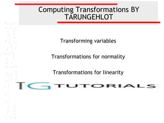
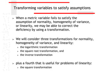
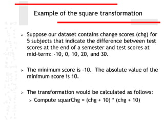
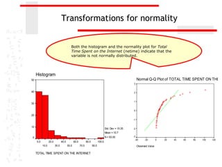
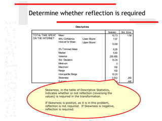
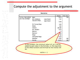
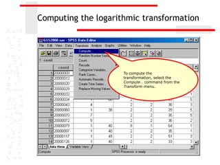
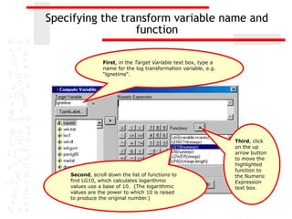
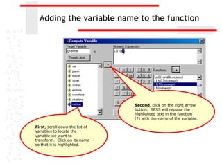
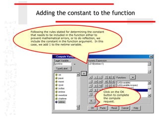
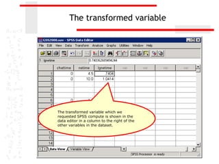
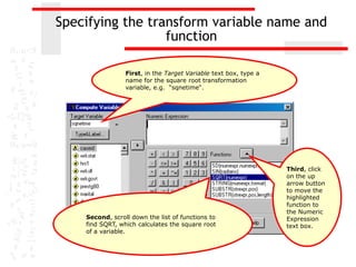
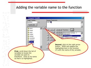
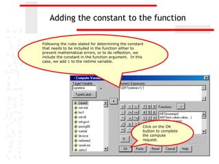
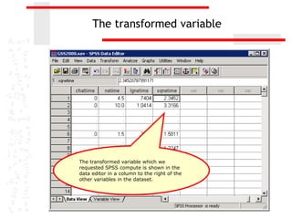
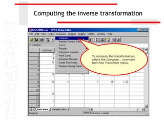
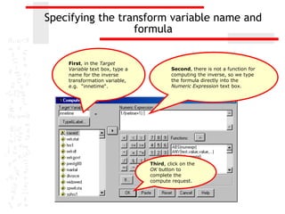
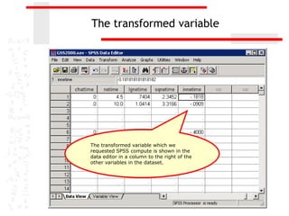
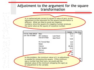
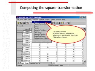
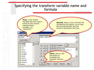
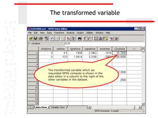
Computing Transformations BY
      TARUNGEHLOT


      Transforming variables

   Transformations for normality

   Transformations for linearity
Transforming variables to satisfy assumptions

   When a metric variable fails to satisfy the
    assumption of normality, homogeneity of variance,
    or linearity, we may be able to correct the
    deficiency by using a transformation.

   We will consider three transformations for normality,
    homogeneity of variance, and linearity:
       the logarithmic transformation
       the square root transformation, and
       the inverse transformation


   plus a fourth that is useful for problems of linearity:
       the square transformation
Computing transformations in SPSS

   In SPSS, transformations are obtained by computing a
    new variable. SPSS functions are available for the
    logarithmic (LG10) and square root (SQRT)
    transformations. The inverse transformation uses a
    formula which divides one by the original value for
    each case.

   For each of these calculations, there may be data
    values which are not mathematically permissible.
    For example, the log of zero is not defined
    mathematically, division by zero is not permitted,
    and the square root of a negative number results in
    an “imaginary” value. We will usually adjust the
    values passed to the function to make certain that
    these illegal operations do not occur.
Two forms for computing transformations

   There are two forms for each of the transformations
    to induce normality, depending on whether the
    distribution is skewed negatively to the left or
    skewed positively to the right.

   Both forms use the same SPSS functions and formula
    to calculate the transformations.

   The two forms differ in the value or argument passed
    to the functions and formula. The argument to the
    functions is an adjustment to the original value of
    the variable to make certain that all of the
    calculations are mathematically correct.
Functions and formulas for transformations

   Symbolically, if we let x stand for the argument
    passes to the function or formula, the calculations
    for the transformations are:
       Logarithmic transformation: compute log =
        LG10(x)
       Square root transformation: compute sqrt =
        SQRT(x)
       Inverse transformation: compute inv = 1 / (x)
       Square transformation: compute s2 = x * x
   For all transformations, the argument must be
    greater than zero to guarantee that the calculations
    are mathematically legitimate.
Transformation of positively skewed variables

   For positively skewed variables, the argument is an
    adjustment to the original value based on the
    minimum value for the variable.

   If the minimum value for a variable is zero, the
    adjustment requires that we add one to each value,
    e.g. x + 1.

   If the minimum value for a variable is a negative
    number (e.g., –6), the adjustment requires that we
    add the absolute value of the minimum value (e.g. 6)
    plus one (e.g. x + 6 + 1, which equals x +7).
Example of positively skewed variable


   Suppose our dataset contains the number of books
    read (books) for 5 subjects: 1, 3, 0, 5, and 2, and the
    distribution is positively skewed.

   The minimum value for the variable books is 0. The
    adjustment for each case is books + 1.

   The transformations would be calculated as follows:
      Compute logBooks = LG10(books + 1)

      Compute sqrBooks = SQRT(books + 1)

      Compute invBooks = 1 / (books + 1)
Transformation of negatively skewed variables


   If the distribution of a variable is negatively skewed,
    the adjustment of the values reverses, or reflects,
    the distribution so that it becomes positively
    skewed. The transformations are then computed on
    the values in the positively skewed distribution.

   Reflection is computed by subtracting all of the
    values for a variable from one plus the absolute
    value of maximum value for the variable. This results
    in a positively skewed distribution with all values
    larger than zero.
Example of negatively skewed variable


   Suppose our dataset contains the number of books
    read (books) for 5 subjects: 1, 3, 0, 5, and 2, and the
    distribution is negatively skewed.

   The maximum value for the variable books is 5. The
    adjustment for each case is 6 - books.

   The transformations would be calculated as follows:
      Compute logBooks = LG10(6 - books)

      Compute sqrBooks = SQRT(6 - books)

      Compute invBooks = 1 / (6 - books)
The Square Transformation for Linearity


   The square transformation is computed by
    multiplying the value for the variable by itself.

   It does not matter whether the distribution is
    positively or negatively skewed.

   It does matter if the variable has negative values,
    since we would not be able to distinguish their
    squares from the square of a comparable positive
    value (e.g. the square of -4 is equal to the square of
    +4). If the variable has negative values, we add the
    absolute value of the minimum value to each score
    before squaring it.
Example of the square transformation


   Suppose our dataset contains change scores (chg) for
    5 subjects that indicate the difference between test
    scores at the end of a semester and test scores at
    mid-term: -10, 0, 10, 20, and 30.

   The minimum score is -10. The absolute value of the
    minimum score is 10.

   The transformation would be calculated as follows:
      Compute squarChg = (chg + 10) * (chg + 10)
Transformations for normality


                                                      Both the histogram and the normality plot for Total
                                                      Time Spent on the Internet (netime) indicate that the
                                                      variable is not normally distributed.


                 Histogram
            50                                                                                                        Normal Q-Q Plot of TOTAL TIME SPENT ON THE IN
                                                                                                                 3


            40                                                                                                   2


                                                                                                                 1
            30

                                                                                                                 0

            20
                                                                                              Expected Normal


                                                                                                                 -1
Frequency


            10
                                                                                              Std. Dev = 15.35   -2
                                                                                              Mean = 10.7
                                                                                              N = 93.00          -3
            0
                                                                                                                   -40      -20        0   20   40   60   80   100   120
                 0.0          20.0          40.0          60.0          80.0          100.0
                       10.0          30.0          50.0          70.0          90.0                                   Observed Value

                 TOTAL TIME SPENT ON THE INTERNET
Determine whether reflection is required
                                     Descriptives

                                                         Stat istic   Std. Error
 TOTAL TIME SPENT   Mean                                     10.73          1.59
 ON THE INTERNET    95% Confidence         Lower Bound         7.57
                    Interval for Mean      Upper Bound
                                                             13.89

                    5% Trimmed Mean                          8.29
                    Median                                   5.50
                    Variance                              235. 655
                    Std. Deviation                          15.35
                    Minimum                                      0
                    Maximum                                    102
                    Range                                      102
                    Interquartile Range                     10.20
                    Skewness                                3.532          .250
                    Kurt osis                              15.614          .495


         Skewness, in the table of Descriptive Statistics,
         indicates whether or not reflection (reversing the
         values) is required in the transformation.

         If Skewness is positive, as it is in this problem,
         reflection is not required. If Skewness is negative,
         reflection is required.
Compute the adjustment to the argument
                                       Descriptives

                                                           Stat istic   Std. Error
   TOTAL TIME SPENT   Mean                                     10.73          1.59
   ON THE INTERNET    95% Confidence         Lower Bound         7.57
                      Interval for Mean      Upper Bound
                                                               13.89

                      5% Trimmed Mean                          8.29
                      Median                                   5.50
                      Variance                              235. 655
                      Std. Deviation                          15.35
                      Minimum                                      0
                      Maximum                                    102
                      Range                                      102
                      Interquartile Range                     10.20
                      Skewness                                3.532          .250
                      Kurt osis                              15.614          .495


          In this problem, the minimum value is 0, so 1 will be
          added to each value in the formula, i.e. the argument
          to the SPSS functions and formula for the inverse will
          be:

                                     netime + 1.
Computing the logarithmic transformation


                     To compute the
                     transformation, select the
                     Compute… command from the
                     Transform menu.
Specifying the transform variable name and
                  function

                 First, in the Target Variable text box, type a
                 name for the log transformation variable, e.g.
                 “lgnetime“.


                                                                  Third, click
                                                                  on the up
                                                                  arrow button
                                                                  to move the
                                                                  highlighted
                                                                  function to
    Second, scroll down the list of functions to                  the Numeric
    find LG10, which calculates logarithmic                       Expression
    values use a base of 10. (The logarithmic                     text box.
    values are the power to which 10 is raised
    to produce the original number.)
Adding the variable name to the function


                                 Second, click on the right arrow
                                 button. SPSS will replace the
                                 highlighted text in the function
                                 (?) with the name of the variable.

First, scroll down the list of
variables to locate the
variable we want to
transform. Click on its name
so that it is highlighted.
Adding the constant to the function

Following the rules stated for determining the constant
that needs to be included in the function either to
prevent mathematical errors, or to do reflection, we
include the constant in the function argument. In this
case, we add 1 to the netime variable.


                                                      Click on the OK
                                                      button to complete
                                                      the compute
                                                      request.
The transformed variable


The transformed variable which we
requested SPSS compute is shown in the
data editor in a column to the right of the
other variables in the dataset.
Computing the square root transformation


                     To compute the transformation,
                     select the Compute… command
                     from the Transform menu.
Specifying the transform variable name and
                  function

                 First, in the Target Variable text box, type a
                 name for the square root transformation
                 variable, e.g. “sqnetime“.


                                                                  Third, click
                                                                  on the up
                                                                  arrow button
                                                                  to move the
                                                                  highlighted
                                                                  function to
                                                                  the Numeric
    Second, scroll down the list of functions to                  Expression
    find SQRT, which calculates the square root                   text box.
    of a variable.
Adding the variable name to the function


                                 Second, click on the right arrow
                                 button. SPSS will replace the
                                 highlighted text in the function
                                 (?) with the name of the variable.
First, scroll down the list of
variables to locate the
variable we want to
transform. Click on its name
so that it is highlighted.
Adding the constant to the function

Following the rules stated for determining the constant
that needs to be included in the function either to
prevent mathematical errors, or to do reflection, we
include the constant in the function argument. In this
case, we add 1 to the netime variable.


                                                      Click on the OK
                                                      button to complete
                                                      the compute
                                                      request.
The transformed variable


The transformed variable which we
requested SPSS compute is shown in the
data editor in a column to the right of the
other variables in the dataset.
Computing the inverse transformation


                   To compute the transformation,
                   select the Compute… command
                   from the Transform menu.
Specifying the transform variable name and
                  formula

    First, in the Target
    Variable text box, type a            Second, there is not a function for
    name for the inverse                 computing the inverse, so we type
    transformation variable,             the formula directly into the
    e.g. “innetime“.                     Numeric Expression text box.


                                Third, click on the
                                OK button to
                                complete the
                                compute request.
The transformed variable


The transformed variable which we
requested SPSS compute is shown in the
data editor in a column to the right of the
other variables in the dataset.
Adjustment to the argument for the square
             transformation

    It is mathematically correct to square a value of zero, so the
    adjustment to the argument for the square transformation is
    different. What we need to avoid are negative
    numbers, since the square of a negative number produces
    the same value as the square of a positive number.
                                      Descriptives

                                                           Stat istic   Std. Error
   TOTAL TIME SPENT   Mean                                     10.73          1.59
   ON THE INTERNET    95% Confidence        Lower Bound          7.57
                      Interval for Mean     Upper Bound
                                                               13.89

                      5% Trimmed Mean                        8.29
                      Median                                 5.50
                      Variance                           235. 655
                      Std. Deviation                        15.35
                      Minimum                                   0
                      Maximum                                 102
                      Range                                   102
                      Interquartile Range                   10.20
    In this problem, the minimum value is 0, no adjustment
                      Skewness                              3.532            .250
    is needed for computing the square. If the minimum
                      Kurt osis                            15.614            .495
    was a number less than zero, we would add the
    absolute value of the minimum (dropping the sign) as
    an adjustment to the variable.
Computing the square transformation


                  To compute the
                  transformation, select the
                  Compute… command from the
                  Transform menu.
Specifying the transform variable name and
                  formula

    First, in the Target
    Variable text box, type a
                                         Second, there is not a function for
    name for the inverse
                                         computing the square, so we type
    transformation
                                         the formula directly into the
    variable, e.g.
                                         Numeric Expression text box.
    “s2netime“.


                                Third, click on the
                                OK button to
                                complete the
                                compute request.
The transformed variable


The transformed variable which we
requested SPSS compute is shown in the
data editor in a column to the right of the
other variables in the dataset.

Computing transformations

  • 1.
    Computing Transformations BY TARUNGEHLOT Transforming variables Transformations for normality Transformations for linearity
  • 2.
    Transforming variables tosatisfy assumptions  When a metric variable fails to satisfy the assumption of normality, homogeneity of variance, or linearity, we may be able to correct the deficiency by using a transformation.  We will consider three transformations for normality, homogeneity of variance, and linearity:  the logarithmic transformation  the square root transformation, and  the inverse transformation  plus a fourth that is useful for problems of linearity:  the square transformation
  • 3.
    Computing transformations inSPSS  In SPSS, transformations are obtained by computing a new variable. SPSS functions are available for the logarithmic (LG10) and square root (SQRT) transformations. The inverse transformation uses a formula which divides one by the original value for each case.  For each of these calculations, there may be data values which are not mathematically permissible. For example, the log of zero is not defined mathematically, division by zero is not permitted, and the square root of a negative number results in an “imaginary” value. We will usually adjust the values passed to the function to make certain that these illegal operations do not occur.
  • 4.
    Two forms forcomputing transformations  There are two forms for each of the transformations to induce normality, depending on whether the distribution is skewed negatively to the left or skewed positively to the right.  Both forms use the same SPSS functions and formula to calculate the transformations.  The two forms differ in the value or argument passed to the functions and formula. The argument to the functions is an adjustment to the original value of the variable to make certain that all of the calculations are mathematically correct.
  • 5.
    Functions and formulasfor transformations  Symbolically, if we let x stand for the argument passes to the function or formula, the calculations for the transformations are:  Logarithmic transformation: compute log = LG10(x)  Square root transformation: compute sqrt = SQRT(x)  Inverse transformation: compute inv = 1 / (x)  Square transformation: compute s2 = x * x  For all transformations, the argument must be greater than zero to guarantee that the calculations are mathematically legitimate.
  • 6.
    Transformation of positivelyskewed variables  For positively skewed variables, the argument is an adjustment to the original value based on the minimum value for the variable.  If the minimum value for a variable is zero, the adjustment requires that we add one to each value, e.g. x + 1.  If the minimum value for a variable is a negative number (e.g., –6), the adjustment requires that we add the absolute value of the minimum value (e.g. 6) plus one (e.g. x + 6 + 1, which equals x +7).
  • 7.
    Example of positivelyskewed variable  Suppose our dataset contains the number of books read (books) for 5 subjects: 1, 3, 0, 5, and 2, and the distribution is positively skewed.  The minimum value for the variable books is 0. The adjustment for each case is books + 1.  The transformations would be calculated as follows:  Compute logBooks = LG10(books + 1)  Compute sqrBooks = SQRT(books + 1)  Compute invBooks = 1 / (books + 1)
  • 8.
    Transformation of negativelyskewed variables  If the distribution of a variable is negatively skewed, the adjustment of the values reverses, or reflects, the distribution so that it becomes positively skewed. The transformations are then computed on the values in the positively skewed distribution.  Reflection is computed by subtracting all of the values for a variable from one plus the absolute value of maximum value for the variable. This results in a positively skewed distribution with all values larger than zero.
  • 9.
    Example of negativelyskewed variable  Suppose our dataset contains the number of books read (books) for 5 subjects: 1, 3, 0, 5, and 2, and the distribution is negatively skewed.  The maximum value for the variable books is 5. The adjustment for each case is 6 - books.  The transformations would be calculated as follows:  Compute logBooks = LG10(6 - books)  Compute sqrBooks = SQRT(6 - books)  Compute invBooks = 1 / (6 - books)
  • 10.
    The Square Transformationfor Linearity  The square transformation is computed by multiplying the value for the variable by itself.  It does not matter whether the distribution is positively or negatively skewed.  It does matter if the variable has negative values, since we would not be able to distinguish their squares from the square of a comparable positive value (e.g. the square of -4 is equal to the square of +4). If the variable has negative values, we add the absolute value of the minimum value to each score before squaring it.
  • 11.
    Example of thesquare transformation  Suppose our dataset contains change scores (chg) for 5 subjects that indicate the difference between test scores at the end of a semester and test scores at mid-term: -10, 0, 10, 20, and 30.  The minimum score is -10. The absolute value of the minimum score is 10.  The transformation would be calculated as follows:  Compute squarChg = (chg + 10) * (chg + 10)
  • 12.
    Transformations for normality Both the histogram and the normality plot for Total Time Spent on the Internet (netime) indicate that the variable is not normally distributed. Histogram 50 Normal Q-Q Plot of TOTAL TIME SPENT ON THE IN 3 40 2 1 30 0 20 Expected Normal -1 Frequency 10 Std. Dev = 15.35 -2 Mean = 10.7 N = 93.00 -3 0 -40 -20 0 20 40 60 80 100 120 0.0 20.0 40.0 60.0 80.0 100.0 10.0 30.0 50.0 70.0 90.0 Observed Value TOTAL TIME SPENT ON THE INTERNET
  • 13.
    Determine whether reflectionis required Descriptives Stat istic Std. Error TOTAL TIME SPENT Mean 10.73 1.59 ON THE INTERNET 95% Confidence Lower Bound 7.57 Interval for Mean Upper Bound 13.89 5% Trimmed Mean 8.29 Median 5.50 Variance 235. 655 Std. Deviation 15.35 Minimum 0 Maximum 102 Range 102 Interquartile Range 10.20 Skewness 3.532 .250 Kurt osis 15.614 .495 Skewness, in the table of Descriptive Statistics, indicates whether or not reflection (reversing the values) is required in the transformation. If Skewness is positive, as it is in this problem, reflection is not required. If Skewness is negative, reflection is required.
  • 14.
    Compute the adjustmentto the argument Descriptives Stat istic Std. Error TOTAL TIME SPENT Mean 10.73 1.59 ON THE INTERNET 95% Confidence Lower Bound 7.57 Interval for Mean Upper Bound 13.89 5% Trimmed Mean 8.29 Median 5.50 Variance 235. 655 Std. Deviation 15.35 Minimum 0 Maximum 102 Range 102 Interquartile Range 10.20 Skewness 3.532 .250 Kurt osis 15.614 .495 In this problem, the minimum value is 0, so 1 will be added to each value in the formula, i.e. the argument to the SPSS functions and formula for the inverse will be: netime + 1.
  • 15.
    Computing the logarithmictransformation To compute the transformation, select the Compute… command from the Transform menu.
  • 16.
    Specifying the transformvariable name and function First, in the Target Variable text box, type a name for the log transformation variable, e.g. “lgnetime“. Third, click on the up arrow button to move the highlighted function to Second, scroll down the list of functions to the Numeric find LG10, which calculates logarithmic Expression values use a base of 10. (The logarithmic text box. values are the power to which 10 is raised to produce the original number.)
  • 17.
    Adding the variablename to the function Second, click on the right arrow button. SPSS will replace the highlighted text in the function (?) with the name of the variable. First, scroll down the list of variables to locate the variable we want to transform. Click on its name so that it is highlighted.
  • 18.
    Adding the constantto the function Following the rules stated for determining the constant that needs to be included in the function either to prevent mathematical errors, or to do reflection, we include the constant in the function argument. In this case, we add 1 to the netime variable. Click on the OK button to complete the compute request.
  • 19.
    The transformed variable Thetransformed variable which we requested SPSS compute is shown in the data editor in a column to the right of the other variables in the dataset.
  • 20.
    Computing the squareroot transformation To compute the transformation, select the Compute… command from the Transform menu.
  • 21.
    Specifying the transformvariable name and function First, in the Target Variable text box, type a name for the square root transformation variable, e.g. “sqnetime“. Third, click on the up arrow button to move the highlighted function to the Numeric Second, scroll down the list of functions to Expression find SQRT, which calculates the square root text box. of a variable.
  • 22.
    Adding the variablename to the function Second, click on the right arrow button. SPSS will replace the highlighted text in the function (?) with the name of the variable. First, scroll down the list of variables to locate the variable we want to transform. Click on its name so that it is highlighted.
  • 23.
    Adding the constantto the function Following the rules stated for determining the constant that needs to be included in the function either to prevent mathematical errors, or to do reflection, we include the constant in the function argument. In this case, we add 1 to the netime variable. Click on the OK button to complete the compute request.
  • 24.
    The transformed variable Thetransformed variable which we requested SPSS compute is shown in the data editor in a column to the right of the other variables in the dataset.
  • 25.
    Computing the inversetransformation To compute the transformation, select the Compute… command from the Transform menu.
  • 26.
    Specifying the transformvariable name and formula First, in the Target Variable text box, type a Second, there is not a function for name for the inverse computing the inverse, so we type transformation variable, the formula directly into the e.g. “innetime“. Numeric Expression text box. Third, click on the OK button to complete the compute request.
  • 27.
    The transformed variable Thetransformed variable which we requested SPSS compute is shown in the data editor in a column to the right of the other variables in the dataset.
  • 28.
    Adjustment to theargument for the square transformation It is mathematically correct to square a value of zero, so the adjustment to the argument for the square transformation is different. What we need to avoid are negative numbers, since the square of a negative number produces the same value as the square of a positive number. Descriptives Stat istic Std. Error TOTAL TIME SPENT Mean 10.73 1.59 ON THE INTERNET 95% Confidence Lower Bound 7.57 Interval for Mean Upper Bound 13.89 5% Trimmed Mean 8.29 Median 5.50 Variance 235. 655 Std. Deviation 15.35 Minimum 0 Maximum 102 Range 102 Interquartile Range 10.20 In this problem, the minimum value is 0, no adjustment Skewness 3.532 .250 is needed for computing the square. If the minimum Kurt osis 15.614 .495 was a number less than zero, we would add the absolute value of the minimum (dropping the sign) as an adjustment to the variable.
  • 29.
    Computing the squaretransformation To compute the transformation, select the Compute… command from the Transform menu.
  • 30.
    Specifying the transformvariable name and formula First, in the Target Variable text box, type a Second, there is not a function for name for the inverse computing the square, so we type transformation the formula directly into the variable, e.g. Numeric Expression text box. “s2netime“. Third, click on the OK button to complete the compute request.
  • 31.
    The transformed variable Thetransformed variable which we requested SPSS compute is shown in the data editor in a column to the right of the other variables in the dataset.