This document summarizes key concepts in probability and Bayesian statistics:
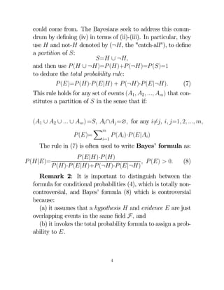
1) It defines conditional probability as the probability of event A given event B. Bayes' theorem is derived from the formula for conditional probability by interpreting events as hypotheses and evidence.
2) Bayes' theorem provides a formula for calculating the posterior probability of a hypothesis given observed evidence by combining the prior probability, likelihood, and evidence probability.
3) Bayesian confirmation theory assesses whether evidence confirms or disconfirms a hypothesis by comparing the hypothesis' prior and posterior probabilities given the evidence. Several measures are provided to quantify the degree of confirmation.
![PHIL 6334 - Probability/Statistics Lecture Notes 2:
Conditional Probabilities and Bayes’ theorem
Aris Spanos [Spring 2014]
1
The view from the ( F ()) perspective
1.1
Conditional probability
Consider the probability set up described by the probability
space ( F ()) where - set of all possible outcomes, F field of events of interest, and () a probability set function
assigning probabilities to events in F
For any two events and in F the following formula for
conditional probability holds:
(|)=
( ∩ )
() 0
()
(1)
This formula treats the events and symmetrically, and
thus:
( ∩ )
() 0
(2)
(|)=
()
Solving (1) and (2) for ( ∩ ) yields the multiplication
rule:
( ∩ )= (|)· ()= (|)· ()
(3)
Substituting (3) into (1) yields the conditional probability:
(|)=
(|)· ()
() 0
()
1
(4)](https://image.slidesharecdn.com/6334-spanos-lecture-2-140208152317-phpapp01/85/6334-Day-3-slides-Spanos-lecture-2-1-320.jpg)
![PHIL 6334 - Probability/Statistics Lecture Notes 2:
Conditional Probabilities and Bayes’ theorem
Aris Spanos [Spring 2014]
1
The view from the ( F ()) perspective
1.1
Conditional probability
Consider the probability set up described by the probability
space ( F ()) where - set of all possible outcomes, F field of events of interest, and () a probability set function
assigning probabilities to events in F
For any two events and in F the following formula for
conditional probability holds:
(|)=
( ∩ )
() 0
()
(1)
This formula treats the events and symmetrically, and
thus:
( ∩ )
() 0
(2)
(|)=
()
Solving (1) and (2) for ( ∩ ) yields the multiplication
rule:
( ∩ )= (|)· ()= (|)· ()
(3)
Substituting (3) into (1) yields the conditional probability:
(|)=
(|)· ()
() 0
()
1
(4)](https://image.slidesharecdn.com/6334-spanos-lecture-2-140208152317-phpapp01/75/6334-Day-3-slides-Spanos-lecture-2-1-2048.jpg)
![Example. Consider the random experiment of tossing a
fair coin twice:
= {() ( ) ( ) ( )}
Let the events of interest be:
= {() ( ) ( )} ()=75
= {( ) ( ) ( )} ()=75
The conditional probability of given takes the form:
(|)=
( ∩ )
=
()
5 2
75 = 3
(5)
since (∩)= (( ) ( ))=5 Notice also that:
(|)=
5 2
75 = 3
→ (∩)= (|)· ()=
5
75 (75)
=5
Now consider introducing a third event:
= {() ( ) ( )} ()=75
What is the conditional probability of given and ?
(| ∩ )=
( ∩ [ ∩ ])
( ∩ ) 0
( ∩ )
which in light of the fact that:
( ∩ )= (|)· () → (|) 0 () 0
(∩)= (() ( ))=5 (∩)= (( ) ( ))=5
(∩∩)= ( )=25 which imply that:
(| ∩ )=
25 1
= (|)=
5
2
2
2
3](https://image.slidesharecdn.com/6334-spanos-lecture-2-140208152317-phpapp01/85/6334-Day-3-slides-Spanos-lecture-2-2-320.jpg)

![1.3
Bayesian Confirmation Theory
The Bayesian confirmation theory relies on comparing the
prior with the posterior probability of hypothesis :
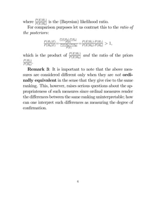
(|) ()
[i] Confirmation:
[ii] Disconfirmation: (|) ()
In case [i] evidence confirms hypothesis , and in case [ii]
evidence disconfirms hypothesis .
The degree of confirmation is measured using some
measure c( ) of the "degree to which raises the probability of ". The most popular such Bayesian measures are:
( )= (|) − ()
( )= (|) − (¬)
( )= (|) − ()
( )= (|) − (¬)
(|)
( )= ()
(|)
( )= (|¬)
One can use any one of the above measures to argue that:
According to measure c( ), evidence favors hypothesis 1 over 0 iff:
c(1 ) c(0 )
For instance using the measure ( ) in the case of two
competing hypotheses 0 and 1 :
(1 |)
(1 )
(0 |) Bayes (|1 )
⇔
(0 )
()
5
(|0 )
()
⇔
(|1 )
(|0 )
1](https://image.slidesharecdn.com/6334-spanos-lecture-2-140208152317-phpapp01/85/6334-Day-3-slides-Spanos-lecture-2-5-320.jpg)