The document discusses image processing in the frequency domain. It covers topics such as the Fourier transform, Hartley transform, and their fast variants. The Fourier transform represents an image as a sum of sine and cosine waves, while the Hartley transform uses only real numbers. Convolution can be performed efficiently in the frequency domain by multiplying the Fourier/Hartley transforms of the image and template and taking the inverse transform. Deconvolution involves finding the inverse of the template to recover the original image from its convolution with the template.

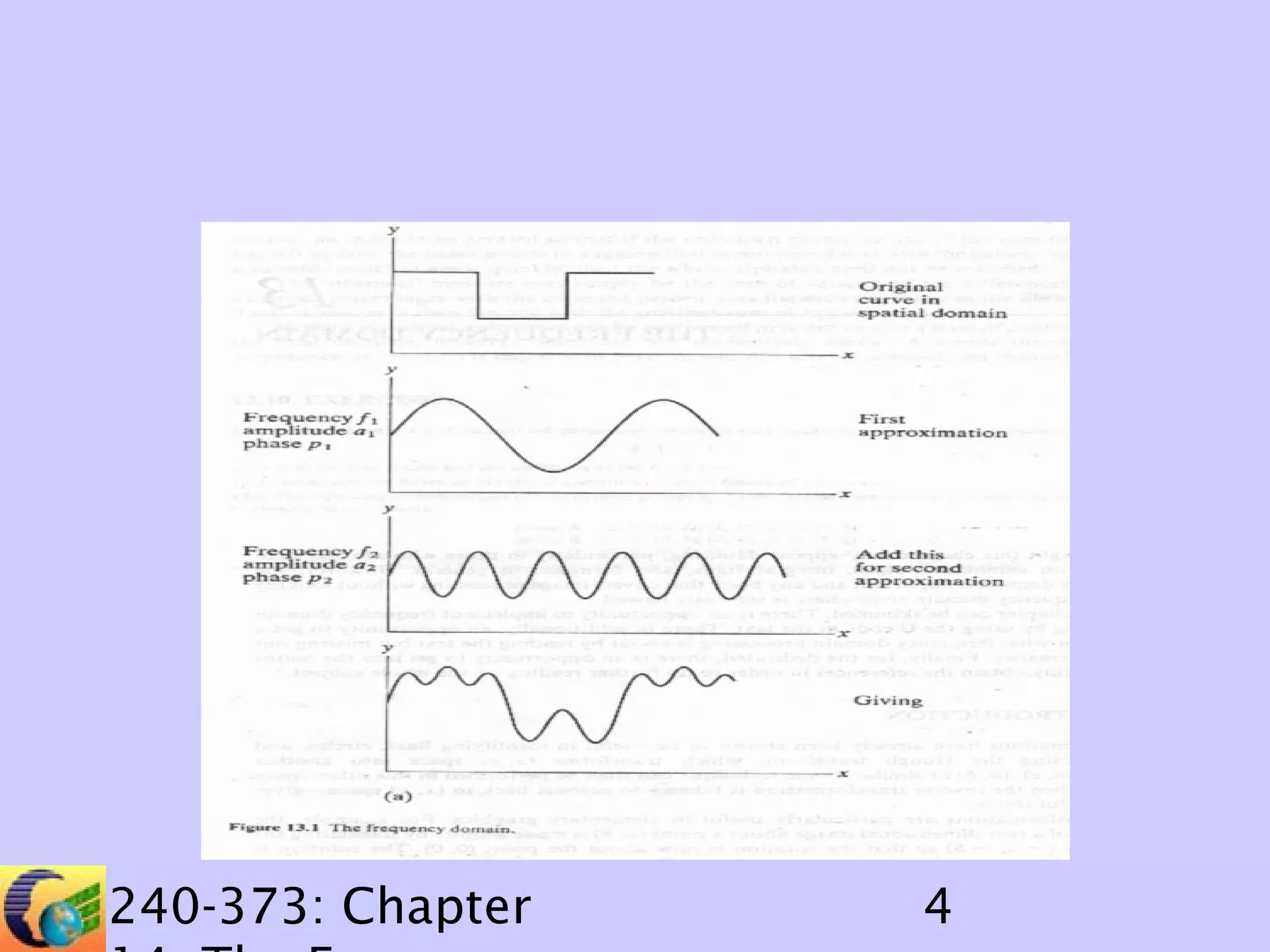
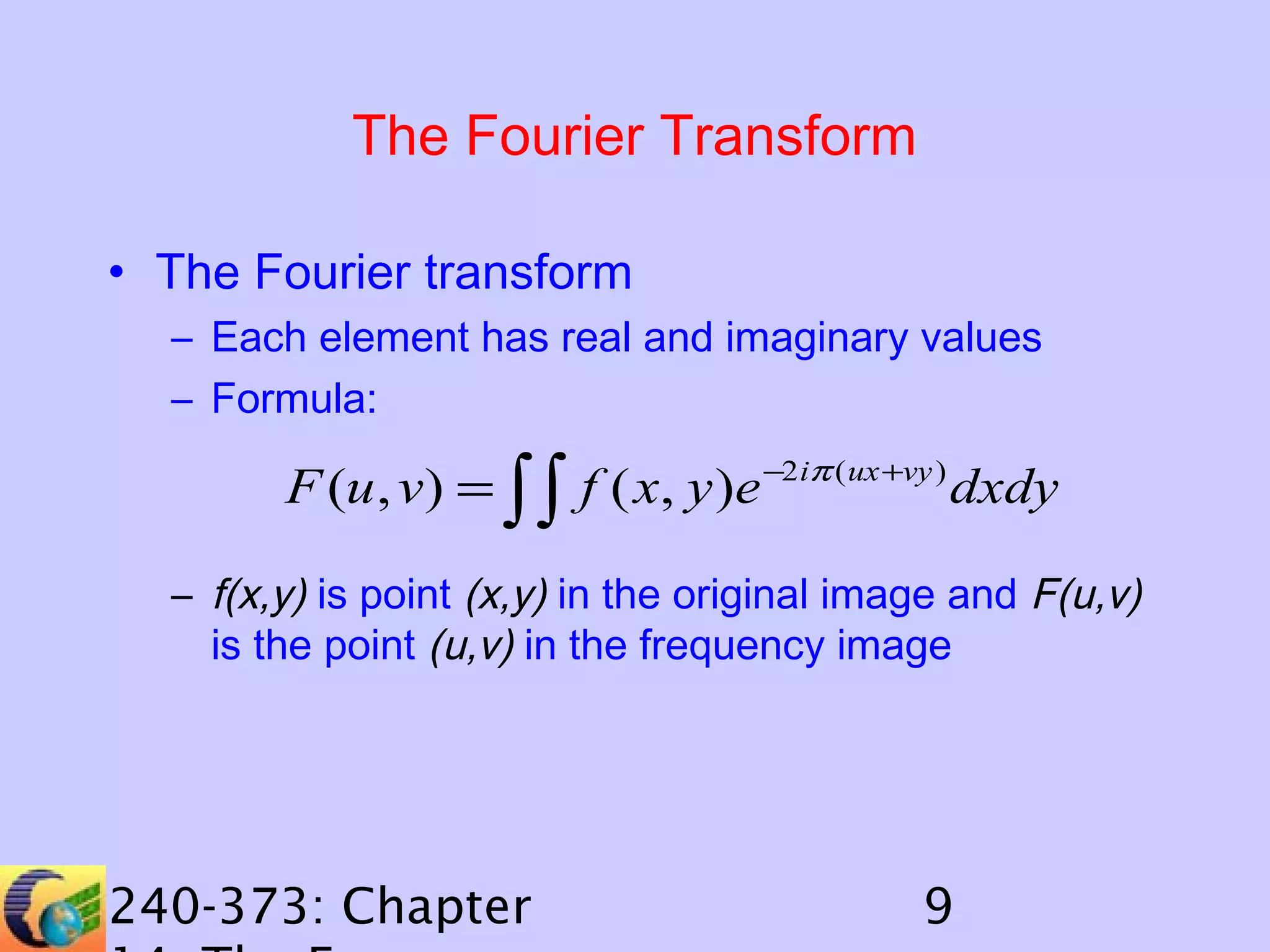
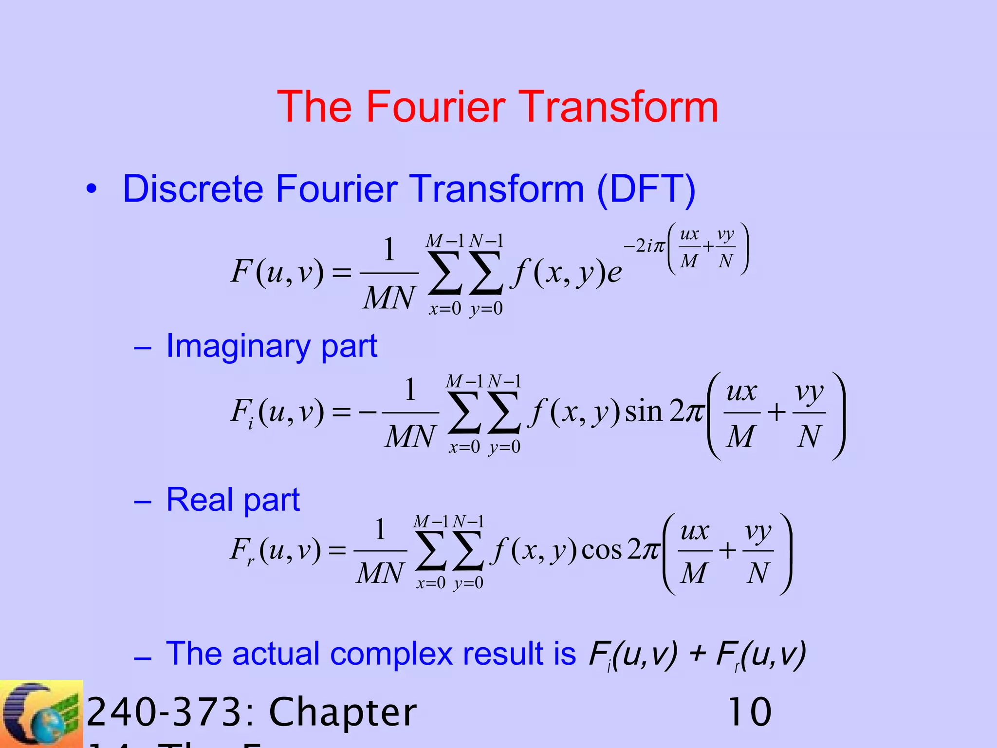
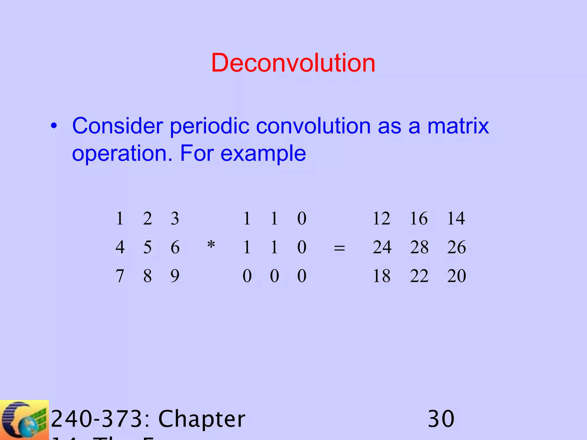
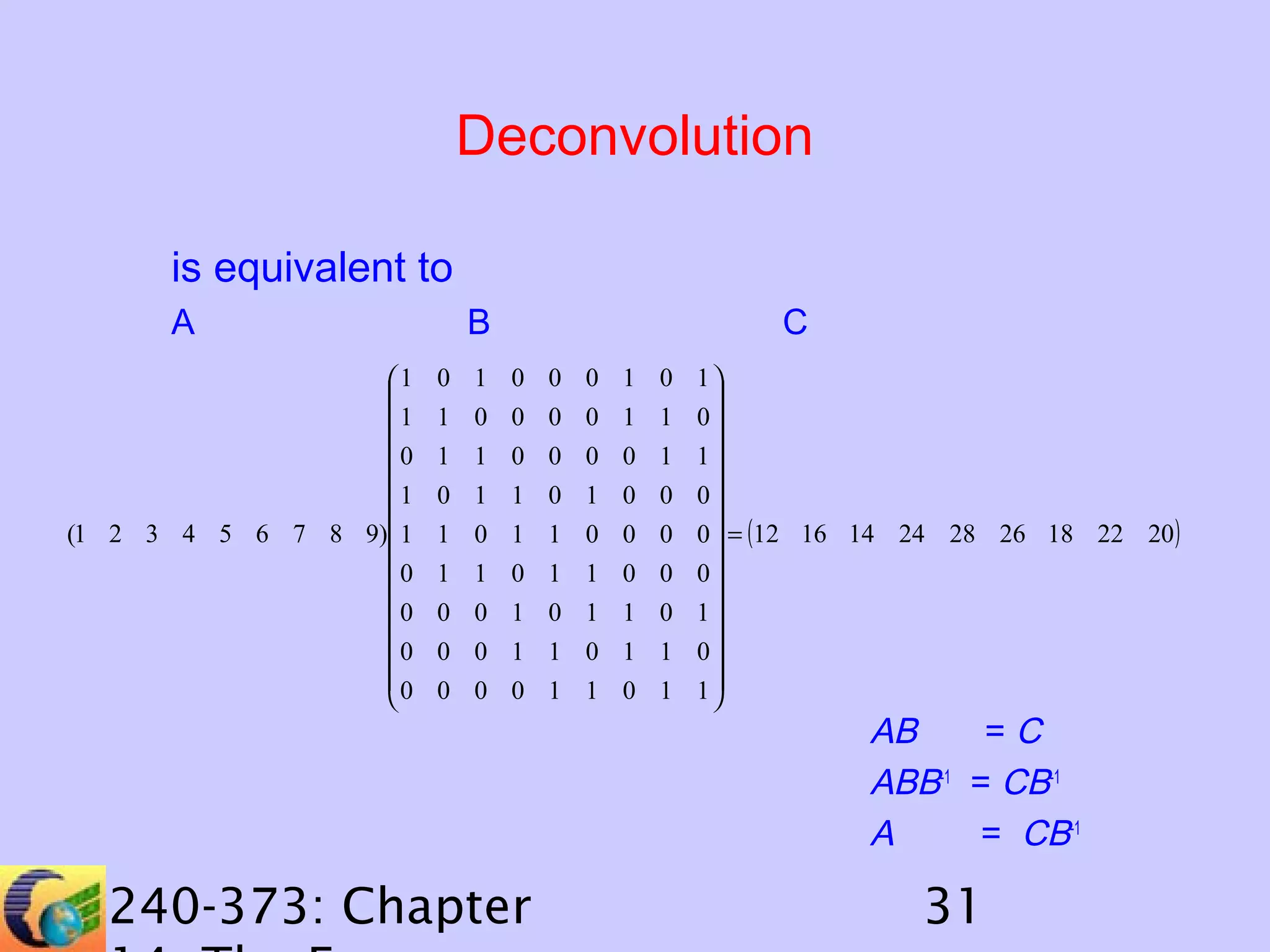
1. 240-373
Image Processing
240-373: Chapter
Montri
Karnjanadecha
montri@coe.psu.ac.t
h
http://
fivedots.coe.psu.ac.t
h/~montri
1

2. Chapter 14
The Frequency
Domain
240-373: Chapter
2

3. The Frequency Domain
• Any wave shape can be approximated by a
sum of periodic (such as sine and cosine)
functions.
• a--amplitude of waveform
• f-- frequency (number of times the wave
repeats itself in a given length)
• p--phase (position that the wave starts)
• Usually phase is ignored in image processing
240-373: Chapter
3

4. 240-373: Chapter
4

5. 240-373: Chapter
5

6. The Hartley Transform
• Discrete Hartley Transform (DHT)
– The M x N image is converted into a second
image (also M x N)
– M and N should be power of 2 (e.g. .., 128, 256,
512, etc.)
– The basic transform depends on calculating the
following for each pixel in the new M x N array
1
H (u , v) =
MN
M −1 N −1
∑∑
x =0 y =0

 ux vy 
 ux vy 
f ( x, y ) ⋅ cos(2π ) −  + sin( 2π ) − 
M N 
 M N 

240-373: Chapter
6

7. The Hartley Transform
where f(x,y) is the intensity of the pixel at position
(x,y)
H(u,v) is the value of element in frequency domain
– The results are periodic
– The cosine+sine (CAS) term is call “the kernel of
the transformation” (or ”basis function”)
240-373: Chapter
7

8. The Hartley Transform
• Fast Hartley Transform (FHT)
– M and N must be power of 2
– Much faster than DHT
– Equation:
H (u, v) = { T (u , v) + T ( M − u, v) + T (u , N − v) − T ( M − u , N − v)} / 2
240-373: Chapter
8

9. The Fourier Transform
• The Fourier transform
– Each element has real and imaginary values
– Formula:
F (u , v) = ∫∫ f ( x, y )e −2iπ ( ux +vy ) dxdy
– f(x,y) is point (x,y) in the original image and F(u,v)
is the point (u,v) in the frequency image
240-373: Chapter
9

10. The Fourier Transform
• Discrete Fourier Transform (DFT)
 ux vy 
− 2 iπ  + 
1 M −1 N −1
F (u, v) =
f ( x, y )e  M N 
∑∑
MN x =0 y =0
– Imaginary part
1 M −1 N −1
 ux vy 
Fi (u, v) = −
f ( x, y ) sin 2π  + 
∑∑
MN x =0 y =0
M N 
– Real part
1
Fr (u , v) =
MN
M −1 N −1
∑∑
x =0 y =0
 ux vy 
f ( x, y ) cos 2π  + 
M N 
– The actual complex result is Fi(u,v) + Fr(u,v)
240-373: Chapter
10

11. Fourier Power Spectrum and Inverse
Fourier Transform
• Fourier power spectrum
F (u , v) = Fr (u , v) 2 + Fi (u , v) 2
• Inverse Fourier Transform
1
f ( x, y ) =
MN
240-373: Chapter
M −1 N −1
∑∑ F (u, v)e
 ux vy 
2 iπ  + 
M N 
x =0 y =0
11

12. Fourier Power Spectrum and Inverse
Fourier Transform
• Fast Fourier Transform (FFT)
– Much faster than DFT
– M and N must be power of 2
– Computation is reduced from M2N2 to
MN log2 M . log2 N (~1/1000 times)
240-373: Chapter
12

13. Fourier Power Spectrum and Inverse
Fourier Transform
• Optical transformation
– A common approach to view image in frequency
domain
A
D
B
C
Original image
240-373: Chapter
C
B
D
A
Transformed image
13

14. Power and Autocorrelation Functions
• Power function:
[
1
P (u , v) = F (u , v) = H (u , v) 2 + H (−u ,−v) 2
2
• Autocorrelation function
F (u , v)
2
– Inverse Fourier transform of
or
1
[ H (u, v) 2 + H (−u,−v) 2 ]
– Hartley transform of 2
240-373: Chapter
14
]

15. Hartley vs Fourier Transform
240-373: Chapter
15

16. Interpretation of the power function
240-373: Chapter
16

17. Applications of Frequency Domain
Processing
• Convolution in the frequency domain
240-373: Chapter
17

18. Applications of Frequency Domain
Processing
– useful when the image is larger than 1024x1024
and the template size is greater than 16x16
– Template and image must be the same size
1
1 1 1
⇒
1 1 0
0
240-373: Chapter
1
1
0
0
0
0
0
0
0
0
0
0
18

19. – Use FHT or FFT instead of DHT or DFT
– Number of points should be kept small
– The transform is periodic
• zeros must be padded to the image and the template
• minimum image size must be (N+n-1) x (M+m-1)
240-373: Chapter
19

20. 0 1
2
0
4 5 6 0
8 9 10 0
0 0 0 0
240-373: Chapter
1 2 0 0
⊗
45
58
44 12
7 3 0 0
97 110 76 32
=
0 0 0 0
26 29 10 16
0 0 0 0
3 13 14 0
20

21. – Convolution in frequency domain is “real
convolution”
Normal convolution
0 1
2
0
4 5
6
1 2 0 0
0
⊗
8 9 10 0
0 0
0
0
7 3 0 0
0 0 0 0
45
=
0 0 0 0
58
44 12
97 110 76 32
26
29
10 16
3
13
14
0
Real convolution
0
4
8
0
1 2 0
5 6 0
9 10 0
0 0 0
240-373: Chapter
0
0
⊗
0
0
0
0
0
0
0
0
3
2
0
0 1 4 4
0
4 20 33 18
=
7
36 72 85 38
1
56 87 97 30
21

22. Convolution using the Fourier transform
Technique 1: Convolution using the Fourier
transform
USE: To perform a convolution
OPERATION:
– zero-padding both the image (MxN) and the
template (m x n) to the size (N+n-1) x (M+m-1)
– Applying FFT to the modified image and template
– Multiplying element by element of the transformed
image against the transformed template
240-373: Chapter
22

23. Convolution using the Fourier transform
OPERATION: (cont’d)
– Multiplication is done as follows:
F(image)
(r1,i1)
F(template)
F(result)
(r2, i2)
(r1r2 - i1i2, r1i2+r2i1)
i.e. 4 real multiplications and 2 additions
– Performing Inverse Fourier transform
240-373: Chapter
23

24. Hartley convolution
Technique 2: Hartley convolution
USE: To perform a convolution
OPERATION:
– zero-padding both the image (MxN) and the
template (m x n) to the size (N+n-1) x (M+m-1)
image
0 1
2
template
0
1 2 0 0
4 5 6 0
8 9 10 0
0 0 0 0
7 3 0 0
0 0 0 0
0 0 0 0
240-373: Chapter
24

25. Hartley convolution
– Applying Hartley transform to the modified image
and template
image
template
11.25 2.25 3.75 − 5.25
− 2.25 − 3.75 − 0.75 2.75
3.25
3.25
3.75 0.75 1.25 − 1.75
− 9.75 − 0.25 − 3.25 1.25
- 1.75 - 1.75 - 1.25 - 1.25
- 1.75 - 0.25 - 1.25 - 2.75
240-373: Chapter
25
3.25
1.75
0.75
0.75
0.75
2.25

26. Hartley convolution
– Multiplying them by evaluating:
 I (u , v)T (u, v) + I (u , v)T ( N − u , M − v)
NM 

R (u , v) =
+ I ( N − u , M − v)T (u , v)

2 
− I ( N − u , M − v)T ( N − u, M − v)



240-373: Chapter
26

27. Hartley convolution: Cont’d
585
− 33
45
− 213
− 417
75
− 49
39
− 105
− 11 − 25
45
− 27
Giving:
− 59
25
125
– Performing Inverse Hartley transform, gives:
0
1
4
4
4
20 33 18
36 72 85 38
56 87 97 30
240-373: Chapter
27

28. Hartley convolution: Cont’d
240-373: Chapter
28

29. Deconvolution
• Convolution
R = I * T
• Deconvolution I = R *-1 T
• Deconvolution of R by T = convolution of R
• by some ‘inverse’ of the template T (T’)
240-373: Chapter
29

30. Deconvolution
• Consider periodic convolution as a matrix
operation. For example
1 2 3
4 5 6
7 8 9
1 1 0
*
1 1 0
0 0 0
240-373: Chapter
12 16 14
=
24 28 26
18 22 20
30

31. Deconvolution
is equivalent to
A
1

1
0

1
(1 2 3 4 5 6 7 8 9) 1

0

0
0

0

B
C
0 1 0 0 0 1 0 1

1 0 0 0 0 1 1 0
1 1 0 0 0 0 1 1

0 1 1 0 1 0 0 0
1 0 1 1 0 0 0 0  = (12 16 14 24 28 26 18 22 20 )

1 1 0 1 1 0 0 0

0 0 1 0 1 1 0 1
0 0 1 1 0 1 1 0

0 0 0 1 1 0 1 1

240-373: Chapter
AB
=C
ABB-1 = CB-1
A
= CB-1
31