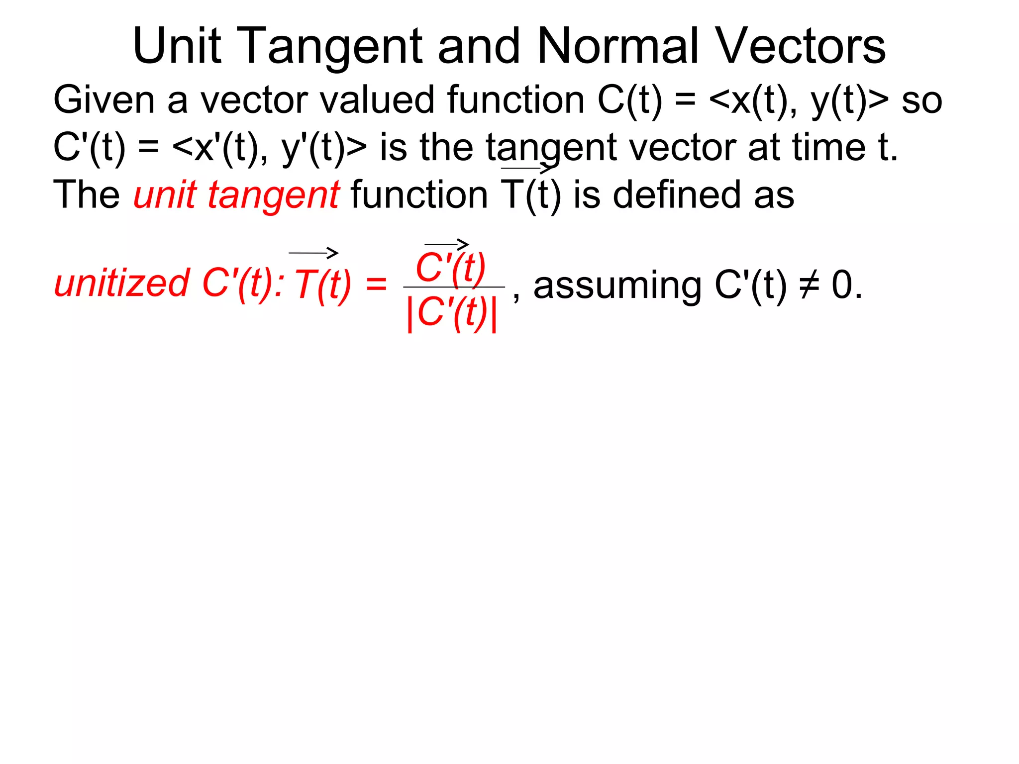
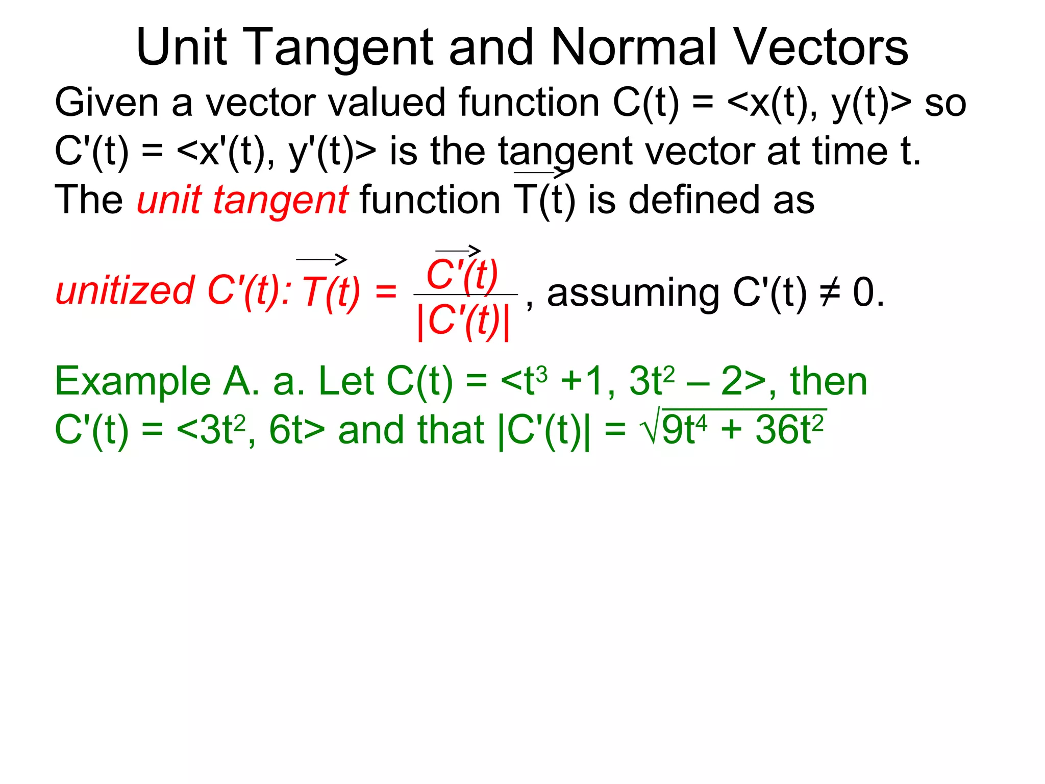
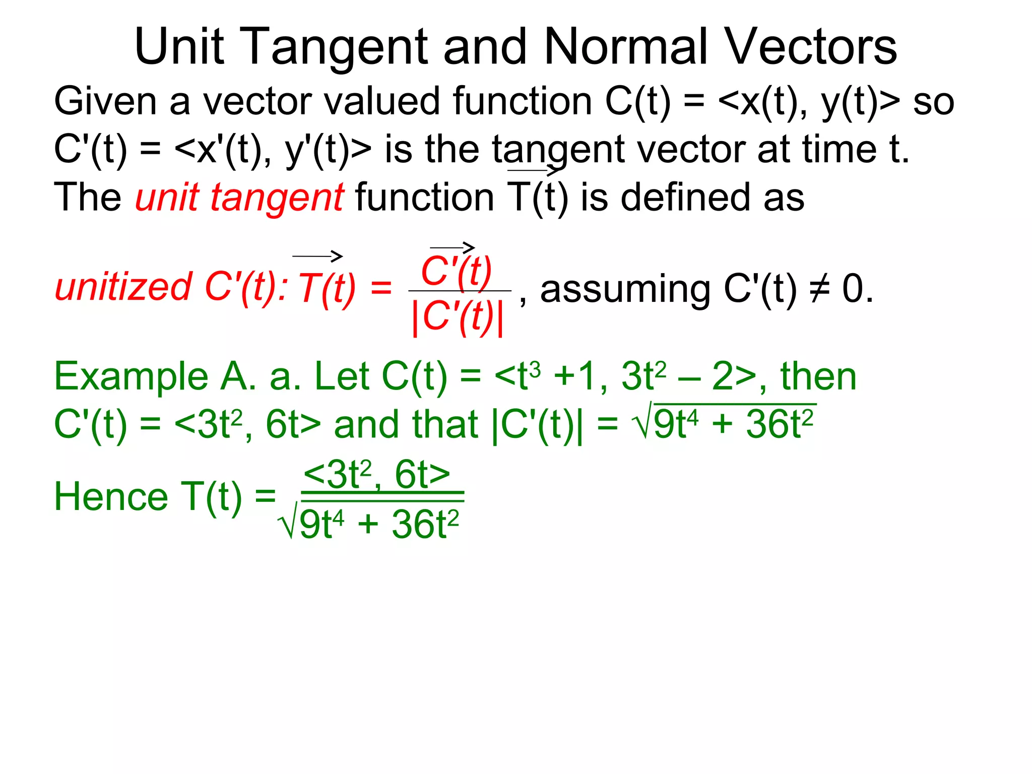
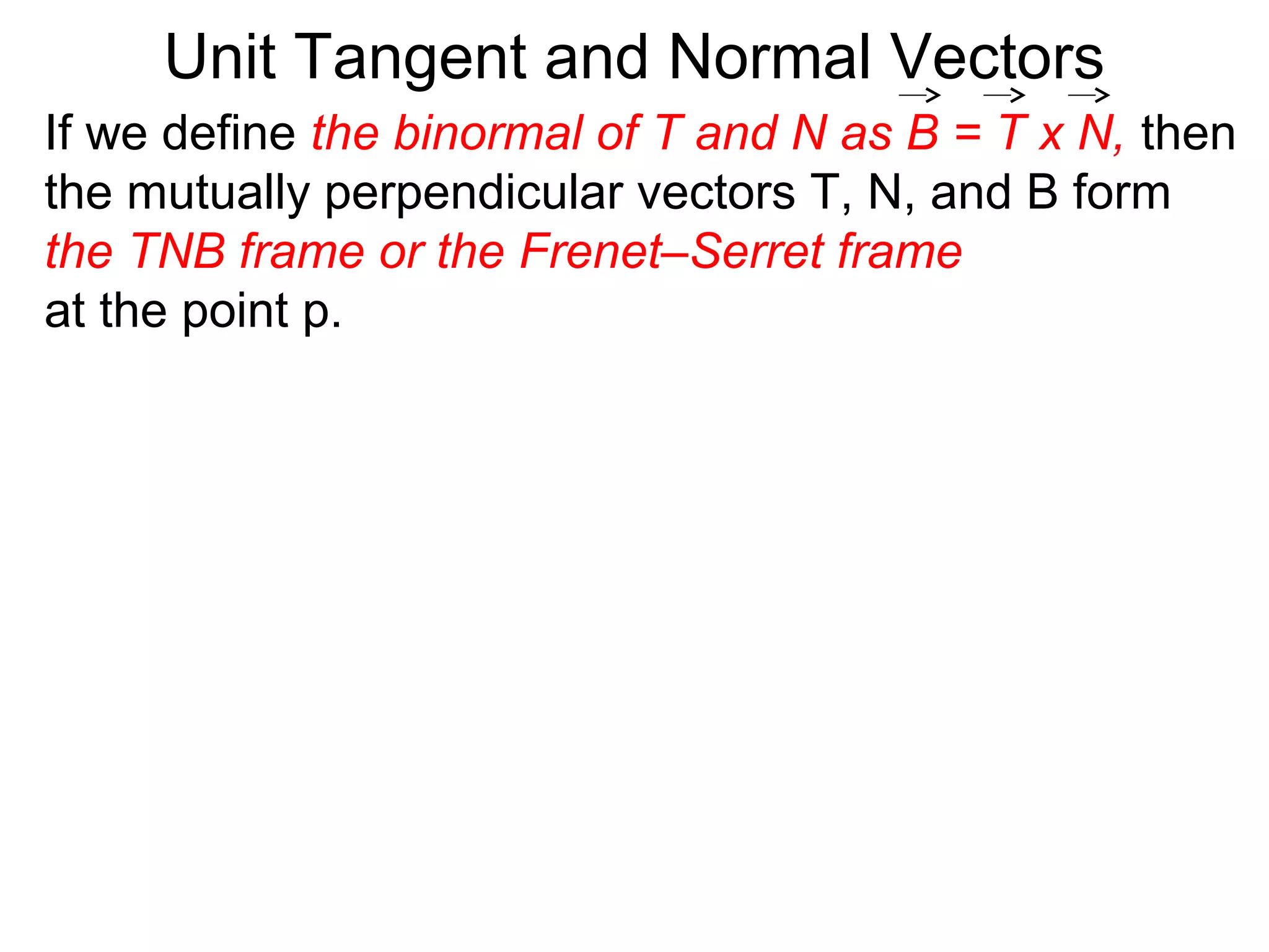
The document defines unit tangent and normal vectors for vector-valued functions. Specifically, it defines the unit tangent vector T(t) as the normalized derivative of the vector-valued function C(t). It also defines the principal normal vector N as the derivative of the unit tangent vector normalized. Finally, it introduces the binormal vector B as the cross product of T and N, forming the Frenet-Serret frame TNB at each point to describe the curve's geometry.

1. Unit Tangent and Normal Vectors

2. Unit Tangent and Normal Vectors
Given a vector valued function C(t) = <x(t), y(t)> so
C'(t) = <x'(t), y'(t)> is the tangent vector at time t.
The unit tangent function T(t) is defined as
unitized C'(t): T(t) = C'(t) , assuming C'(t) ≠ 0.
|C'(t)|

3. Unit Tangent and Normal Vectors
Given a vector valued function C(t) = <x(t), y(t)> so
C'(t) = <x'(t), y'(t)> is the tangent vector at time t.
The unit tangent function T(t) is defined as
unitized C'(t): T(t) = C'(t) , assuming C'(t) ≠ 0.
|C'(t)|
Example A. a. Let C(t) = <t3 +1, 3t2 – 2>, then
C'(t) = <3t2, 6t> and that |C'(t)| = √9t4 + 36t2

4. Unit Tangent and Normal Vectors
Given a vector valued function C(t) = <x(t), y(t)> so
C'(t) = <x'(t), y'(t)> is the tangent vector at time t.
The unit tangent function T(t) is defined as
unitized C'(t): T(t) = C'(t) , assuming C'(t) ≠ 0.
|C'(t)|
Example A. a. Let C(t) = <t3 +1, 3t2 – 2>, then
C'(t) = <3t2, 6t> and that |C'(t)| = √9t4 + 36t2
<3t2, 6t>
Hence T(t) = 4
√9t + 36t2

5. Unit Tangent and Normal Vectors
Given a vector valued function C(t) = <x(t), y(t)> so
C'(t) = <x'(t), y'(t)> is the tangent vector at time t.
The unit tangent function T(t) is defined as
unitized C'(t): T(t) = C'(t) , assuming C'(t) ≠ 0.
|C'(t)|
Example A. a. Let C(t) = <t3 +1, 3t2 – 2>, then
C'(t) = <3t2, 6t> and that |C'(t)| = √9t4 + 36t2
<3t2, 6t>
Hence T(t) = 4
√9t + 36t2
Note that T (t) is undefined when t = 0 at (1, –2).

6. Unit Tangent and Normal Vectors
Given a vector valued function C(t) = <x(t), y(t)> so
C'(t) = <x'(t), y'(t)> is the tangent vector at time t.
The unit tangent function T(t) is defined as
unitized C'(t): T(t) = C'(t) , assuming C'(t) ≠ 0.
|C'(t)|
Example A. a. Let C(t) = <t3 +1, 3t2 – 2>, then
C'(t) = <3t2, 6t> and that |C'(t)| = √9t4 + 36t2
<3t2, 6t>
Hence T(t) = 4
√9t + 36t2
Note that T (t) is undefined when t = 0 at (1, –2).
b. Find C'(1) and T (1).

7. Unit Tangent and Normal Vectors
Given a vector valued function C(t) = <x(t), y(t)> so
C'(t) = <x'(t), y'(t)> is the tangent vector at time t.
The unit tangent function T(t) is defined as
unitized C'(t): T(t) = C'(t) , assuming C'(t) ≠ 0.
|C'(t)|
Example A. a. Let C(t) = <t3 +1, 3t2 – 2>, then
C'(t) = <3t2, 6t> and that |C'(t)| = √9t4 + 36t2
<3t2, 6t>
Hence T(t) = 4
√9t + 36t2
Note that T (t) is undefined when t = 0 at (1, –2).
b. Find C'(1) and T (1).
C'(1) = <3, 6>,

8. Unit Tangent and Normal Vectors
The principal unit normal vector is defined as:
T'(t)
N= = the derivative of T unitized
|T'(t)|
Because |T| = 1 = constant, so T' is normal to T.
Since N is just unitized T' therefore N is also
perpendicular to T
In 2D, there are two unit normal vectors to the curve C,
i.e. perpendicular to the tangent C'(t) (or T).
T
N is the normal vector that is in the
direction the curve is turning.
N

9. Unit Tangent and Normal Vectors
More pecisely, given a vector u = <a, b> in 2D, the
vectors <-b, a> and <b, -a> are normal to u.

10. Unit Tangent and Normal Vectors
More pecisely, given a vector u = <a, b> in 2D, the
vectors <-b, a> and <b, -a> are normal to u.
<-b, a> is in the counter-clockwise direction.

11. Unit Tangent and Normal Vectors
More pecisely, given a vector u = <a, b> in 2D, the
vectors <-b, a> and <b, -a> are normal to u.
<-b, a> is in the counter-clockwise direction.
<b, -a> is in the clockwise direction.

12. Unit Tangent and Normal Vectors
More pecisely, given a vector u = <a, b> in 2D, the
vectors <-b, a> and <b, -a> are normal to u.
<-b, a> is in the counter-clockwise direction.
<b, -a> is in the clockwise direction.
Example: Given u = <-3, 2>, the vector <-2, -3>
is normal to u in the counter-clockwise direction.
<2, 3> is normal in the clockwise direction.

13. Unit Tangent and Normal Vectors
More pecisely, given a vector u = <a, b> in 2D, the
vectors <-b, a> and <b, -a> are normal to u.
<-b, a> is in the counter-clockwise direction.
<b, -a> is in the clockwise direction.
Example: Given u = <-3, 2>, the vector <-2, -3>
is normal to u in the counter-clockwise direction.
<2, 3> is normal in the clockwise direction.
u=<-3,2>

14. Unit Tangent and Normal Vectors
More pecisely, given a vector u = <a, b> in 2D, the
vectors <-b, a> and <b, -a> are normal to u.
<-b, a> is in the counter-clockwise direction.
<b, -a> is in the clockwise direction.
Example: Given u = <-3, 2>, the vector <-2, -3>
is normal to u in the counter-clockwise direction.
<2, 3> is normal in the clockwise direction.
u=<-3,2>
<-2,-3>

15. Unit Tangent and Normal Vectors
More pecisely, given a vector u = <a, b> in 2D, the
vectors <-b, a> and <b, -a> are normal to u.
<-b, a> is in the counter-clockwise direction.
<b, -a> is in the clockwise direction.
Example: Given u = <-3, 2>, the vector <-2, -3>
is normal to u in the counter-clockwise direction.
<2, 3> is normal in the clockwise direction.
<2,3>
u=<-3,2>
<-2,-3>

16. Unit Tangent and Normal Vectors
More pecisely, given a vector u = <a, b> in 2D, the
vectors <-b, a> and <b, -a> are normal to u.
<-b, a> is in the counter-clockwise direction.
<b, -a> is in the clockwise direction.
Example: Given u = <-3, 2>, the vector <-2, -3>
is normal to u in the counter-clockwise direction.
<2, 3> is normal in the clockwise direction.
Therefore, to find N in 2D, <2,3>
u=<-3,2>
instead of taking deivative,
we just have to decide which
of the two unit normal
vectors is the principlal
<-2,-3>
normal N.

17. Unit Tangent and Normal Vectors
Example: Given C(t) = <t3, t2> and t = -1.
Find the unit tangent T and principal unit normal N
at the given time t. Sketch C(t), T and N

18. Unit Tangent and Normal Vectors
Example: Given C(t) = <t3, t2> and t = -1.
Find the unit tangent T and principal unit normal N
at the given time t. Sketch C(t), T and N
Given that x = t3, y = t2 so x2 = y3.

19. Unit Tangent and Normal Vectors
Example: Given C(t) = <t3, t2> and t = -1.
Find the unit tangent T and principal unit normal N
at the given time t. Sketch C(t), T and N
Given that x = t3, y = t2 so x2 = y3.

20. Unit Tangent and Normal Vectors
Example: Given C(t) = <t3, t2> and t = -1.
Find the unit tangent T and principal unit normal N
at the given time t. Sketch C(t), T and N
Given that x = t3, y = t2 so x2 = y3.
For t = -1, C(-1) = <-1, 1>.
(-1, 1)

21. Unit Tangent and Normal Vectors
Example: Given C(t) = <t3, t2> and t = -1.
Find the unit tangent T and principal unit normal N
at the given time t. Sketch C(t), T and N
Given that x = t3, y = t2 so x2 = y3.
For t = -1, C(-1) = <-1, 1>.
C'(t) = <3t2, 2t> and
|C'(t)| = √9t4 + 4t2
(-1, 1)

22. Unit Tangent and Normal Vectors
Example: Given C(t) = <t3, t2> and t = -1.
Find the unit tangent T and principal unit normal N
at the given time t. Sketch C(t), T and N
Given that x = t3, y = t2 so x2 = y3.
For t = -1, C(-1) = <-1, 1>.
C'(t) = <3t2, 2t> and
|C'(t)| = √9t4 + 4t2
Hence when t =-1, (-1, 1)
T
<3, -2>
T=
√13

23. Unit Tangent and Normal Vectors
Example: Given C(t) = <t3, t2> and t = -1.
Find the unit tangent T and principal unit normal N
at the given time t. Sketch C(t), T and N
Given that x = t3, y = t2 so x2 = y3.
For t = -1, C(-1) = <-1, 1>.
C'(t) = <3t2, 2t> and
|C'(t)| = √9t4 + 4t2
Hence when t =-1, (-1, 1)
T
<3, -2> N
T=
√13
and N = <-2, -3>
√13

24. Unit Tangent and Normal Vectors
Let C(t) = <x(t), y(t), z(t)> be a vector valued function
and let T be the unit tangent at the point p as shown.
p
T

25. Unit Tangent and Normal Vectors
Let C(t) = <x(t), y(t), z(t)> be a vector valued function
and let T be the unit tangent at the point p as shown.
The set of vectors perpendicular to T at p form a plane
M and we define M as the
normal plane to the curve C(t) at p.
p
T

26. Unit Tangent and Normal Vectors
Let C(t) = <x(t), y(t), z(t)> be a vector valued function
and let T be the unit tangent at the point p as shown.
The set of vectors perpendicular to T at p form a plane
M and we define M as the
normal plane to the curve C(t) at p.
p
M
T

27. Unit Tangent and Normal Vectors
Let C(t) = <x(t), y(t), z(t)> be a vector valued function
and let T be the unit tangent at the point p as shown.
The set of vectors perpendicular to T at p form a plane
M and we define M as the
normal plane to the curve C(t) at p.
p
The principal normal N at p is defined as M
N = T'(t) T
|T'(t)|

28. Unit Tangent and Normal Vectors
Let C(t) = <x(t), y(t), z(t)> be a vector valued function
and let T be the unit tangent at the point p as shown.
The set of vectors perpendicular to T at p form a plane
M and we define M as the
normal plane to the curve C(t) at p.
p
The principal normal N at p is defined as M
N = T'(t) T
|T'(t)| Q
This principal normal N is in the
osculating plane, the plane that
is the limit of the plane
p
pQR as Q  p and R p
where Q, R are two other The osculating– T
points on C(t). plane R

29. Unit Tangent and Normal Vectors
Let C(t) = <x(t), y(t), z(t)> be a vector valued function
and let T be the unit tangent at the point p as shown.
The set of vectors perpendicular to T at p form a plane
M and we define M as the
normal plane to the curve C(t) at p.
p
The principal normal N at p is defined as M
N = T'(t) T
|T'(t)| Q
This principal normal N is in the
osculating plane, the plane that
is the limit of the plane N
p
pQR as Q  p and R p
where Q, R are two other The osculating– T
points on C(t). plane R

30. Unit Tangent and Normal Vectors
If we define the binormal of T and N as B = T x N,

31. Unit Tangent and Normal Vectors
If we define the binormal of T and N as B = T x N, then
the mutually perpendicular vectors T, N, and B form
the TNB frame or the Frenet–Serret frame
at the point p.

32. Unit Tangent and Normal Vectors
If we define the binormal of T and N as B = T x N, then
the mutually perpendicular vectors T, N, and B form
the TNB frame or the Frenet–Serret frame
at the point p. The TNB frame with
T: the directional vector
N: unitize left or right turn vector
B: unitize up or down turn vector
is an important system for describing the geometry of
the curve at the point p, independent of its motion
(parameterization).

33. Unit Tangent and Normal Vectors
If we define the binormal of T and N as B = T x N, then
the mutually perpendicular vectors T, N, and B form
the TNB frame or the Frenet–Serret frame
at the point p. The TNB frame with
T: the directional vector
N: unitize left or right turn vector
B: unitize up or down turn vector
is an important system for describing the geometry of
the curve at the point p, independent of its motion
(parameterization). Here are the TNB frames of the
helix as the point travels upward counter–clockwisely.
B
N
T
TNB frames of the helix.

34. Arc length Parameter and Curvature
Given C(t) = <3t +1, 4t – 2>
|C'(t)| = √(x'(t))2 +(y'(t))2 = √32 + 42 = 5,

35. Arc length Parameter and Curvature
Given C(t) = <3t +1, 4t – 2>
|C'(t)| = √(x'(t))2 +(y'(t))2 = √32 + 42 = 5,
so if we calculate its arc–length from t = 0 to t = a,
a a
we have ∫ √(x'(t))2 +(y'(t))2 dt = ∫ 5 dt = 5a.
t=0 t=0

36. Arc length Parameter and Curvature
Given C(t) = <3t +1, 4t – 2>
|C'(t)| = √(x'(t))2 +(y'(t))2 = √32 + 42 = 5,
so if we calculate its arc–length from t = 0 to t = a,
a a
we have ∫ √(x'(t))2 +(y'(t))2 dt = ∫ 5 dt = 5a.
t=0 t=0
For D(t) = <3t/5 +1, 4t/5 – 2>, | D'(t) | = |<3/5, 4/5>| = 1,
a a

37. Arc length Parameter and Curvature
Given C(t) = <3t +1, 4t – 2>
|C'(t)| = √(x'(t))2 +(y'(t))2 = √32 + 42 = 5,
so if we calculate its arc–length from t = 0 to t = a,
a a
we have ∫ √(x'(t))2 +(y'(t))2 dt = ∫ 5 dt = 5a.
t=0 t=0
For D(t) = <3t/5 +1, 4t/5 – 2>, | D'(t) | = |<3/5, 4/5>| = 1,
a a
its length is ∫ √(x'(t))2 +(y'(t))2 dt = ∫ 1 dt = a.
t=0 t=0

38. Arc length Parameter and Curvature
Given C(t) = <3t +1, 4t – 2>
|C'(t)| = √(x'(t))2 +(y'(t))2 = √32 + 42 = 5,
so if we calculate its arc–length from t = 0 to t = a,
a a
we have ∫ √(x'(t))2 +(y'(t))2 dt = ∫ 5 dt = 5a.
t=0 t=0
For D(t) = <3t/5 +1, 4t/5 – 2>, | D'(t) | = |<3/5, 4/5>| = 1,
a a
its length is ∫ √(x'(t))2 +(y'(t))2 dt = ∫ 1 dt = a.
t=0 t=0
C(t) describes a moving particle traveling at the
constant speed of 5 on the line, where as D(t)
describes a particle traveling at a constant speed of 1.

39. Arc length Parameter and Curvature
Given C(t) = <3t +1, 4t – 2>
|C'(t)| = √(x'(t))2 +(y'(t))2 = √32 + 42 = 5,
so if we calculate its arc–length from t = 0 to t = a,
a a
we have ∫ √(x'(t))2 +(y'(t))2 dt = ∫ 5 dt = 5a.
t=0 t=0
For D(t) = <3t/5 +1, 4t/5 – 2>, | D'(t) | = |<3/5, 4/5>| = 1,
a a
its length is ∫ √(x'(t))2 +(y'(t))2 dt = ∫ 1 dt = a.
t=0 t=0
C(t) describes a moving particle traveling at the
constant speed of 5 on the line, where as D(t)
describes a particle traveling at a constant speed of 1.
The parameterization of a curve that corresponds to
a point traveling at a constant speed of 1, such as

40. Arc length Parameter and Curvature
Parametrization by the Arc Length Parameter s
Given a curve and a point p on the curve, we may
parametrize the curve in the following manner:
p

41. Arc length Parameter and Curvature
Parametrization by the Arc Length Parameter s
Given a curve and a point p on the curve, we may
parametrize the curve in the following manner:
Stating at p, select a direction as positive.
+
p

42. Arc length Parameter and Curvature
Parametrization by the Arc Length Parameter s
Given a curve and a point p on the curve, we may
parametrize the curve in the following manner:
Stating at p, select a direction as positive.
Let s be the parameter and <x(s), y(s)> be the
parameterization such that <x(s), y(s)> = q is the
point where the arc–length from p to q is s.
+
p

43. Arc length Parameter and Curvature
Parametrization by the Arc Length Parameter s
Given a curve and a point p on the curve, we may
parametrize the curve in the following manner:
Stating at p, select a direction as positive.
Let s be the parameter and <x(s), y(s)> be the
parameterization such that <x(s), y(s)> = q is the
point where the arc–length from p to q is s.
+
p=<x(0),y(0)>
s=0

44. Arc length Parameter and Curvature
Parametrization by the Arc Length Parameter s
Given a curve and a point p on the curve, we may
parametrize the curve in the following manner:
Stating at p, select a direction as positive.
Let s be the parameter and <x(s), y(s)> be the
parameterization such that <x(s), y(s)> = q is the
point where the arc–length from p to q is s.
+
p=<x(0),y(0)>
s=0
s=1
<x(1),y(1>

45. Arc length Parameter and Curvature
Parametrization by the Arc Length Parameter s
Given a curve and a point p on the curve, we may
parametrize the curve in the following manner:
Stating at p, select a direction as positive.
Let s be the parameter and <x(s), y(s)> be the
parameterization such that <x(s), y(s)> = q is the
point where the arc–length from p to q is s.
+
p=<x(0),y(0)>
s=0
s=2
s=1 <x(2),y(2>
<x(1),y(1>

46. Arc length Parameter and Curvature
Parametrization by the Arc Length Parameter s
Given a curve and a point p on the curve, we may
parametrize the curve in the following manner:
Stating at p, select a direction as positive.
Let s be the parameter and <x(s), y(s)> be the
parameterization such that <x(s), y(s)> = q is the
point where the arc–length from p to q is s.
+
p=<x(0),y(0)> s=3
<x(3),y(3>
s=0
s=2
s=1 <x(2),y(2>
<x(1),y(1>

47. Arc length Parameter and Curvature
Parametrization by the Arc Length Parameter s
Given a curve and a point p on the curve, we may
parametrize the curve in the following manner:
Stating at p, select a direction as positive.
Let s be the parameter and <x(s), y(s)> be the
parameterization such that <x(s), y(s)> = q is the
point where the arc–length from p to q is s.
+
s=-1 p=<x(0),y(0)> s=3
s=-2 <x(3),y(3>
s=0
s=2
s=-3 s=1 <x(2),y(2>
<x(1),y(1>

48. Arc length Parameter and Curvature
Parametrization by the Arc Length Parameter s
Given a curve and a point p on the curve, we may
parametrize the curve in the following manner:
Stating at p, select a direction as positive.
Let s be the parameter and <x(s), y(s)> be the
parameterization such that <x(s), y(s)> = q is the
point where the arc–length from p to q is s.
q=<x(s),y(s)>
+
arc–length=s
s=-1 p=<x(0),y(0)> s=3
s=-2 <x(3),y(3>
s=0
s=2
s=-3 s=1 <x(2),y(2>
<x(1),y(1>

49. Parametrized by Arc length
Parametrization by the Arc Length Parameter s
Given a curve and a point p on the curve, we may
parametrize the curve in the following manner:
Stating at p, select a direction as positive.
Let s be the parameter and <x(s), y(s)> be the
parameterization such that <x(s), y(s)> = q is the
point where the arc–length from p to q is s.
3 s + 1, 4 s – 2 q=<x(s),y(s)>
For example, D(s) =< 5 5 >
+
is parametrized by the arc-length s
arc–length=s
since | dD | = 1.
ds s=-1 p=<x(0),y(0)> s=3
s=-2 <x(3),y(3>
The starting point of D s=0
s=2
is p = D(0) = (1, –2). s=-3 s=1 <x(2),y(2>
<x(1),y(1>

50. Parametrized by Arc length
Fact: Given a differentiable curve C(t) = <x(t), y(t)>,
(C'(t) ≠ 0) and a point p on C, we may reparametrize
the curve C(t) as D(s) = <x(s), y(s)>
such that |dD/ds| = 1 (Note the derivative here is with
respect to s, not t.). Save for a few examples like the
one above, given a C(t) = <x(t), y(t)>, the actual
calculation of D(s) = <x(s), y(s)> yields non–elementary
functions i.e. it’s not doable. However the importance
of the above fact is that D(s) = <x(s), y(s)> exists.
Since C(t) and D(s) produce the curve, geometric
measurements may be defined easier using
D(s) = <x(s), y(s)>. But the actual calculation of such
measurements will be done directly from the given C(t)
at hand without actually computing D(s).

51. Parametrized by Arc length
If we are blindfolded sitting in a moving car on a curvy
road but we are able to determine how fast and how
sharp the turn is at each point on the road, then
theoretically we may reconstruct the layout of the road.
However, the geometry or the shape of the road is
independent from the actual trip, i.e. different trips
should yield the same reconstructed shape for the
road. to determine the curviness or the curvature at a
Hence
point p on C(t) = <x(t), y(t)>, we first reparametrized
C(t) by the curve length as D(s) = <x(s), y(s)>
so that |D(s)/ds| = 1, i.e. D(s) represents a motion with
speed = 1. Then we use the acceleration vector of
D(s), which gives the change in the unit–tangent T (=
D'(s) ),

52. Vector-valued Functions
Let D(s) = <x(s), y(s)> be parametrized by the
arc– length so |dD(s)/ds| = 1. Hence dD(s)/ds = T(s)
the unit tangent of D(s), and that dT/ds is perpendicular
to T in the direction of the principal normal N to the
curve, thus dD/ds = κN for some κ. The number
κ measures the rate the curve is making turn and is
defined to be the curvature at the point.
y
x
A curve with constant norm A curve with constant norm
in R2 and its tangent in R3 and its tangent