Download as PDF, PPTX

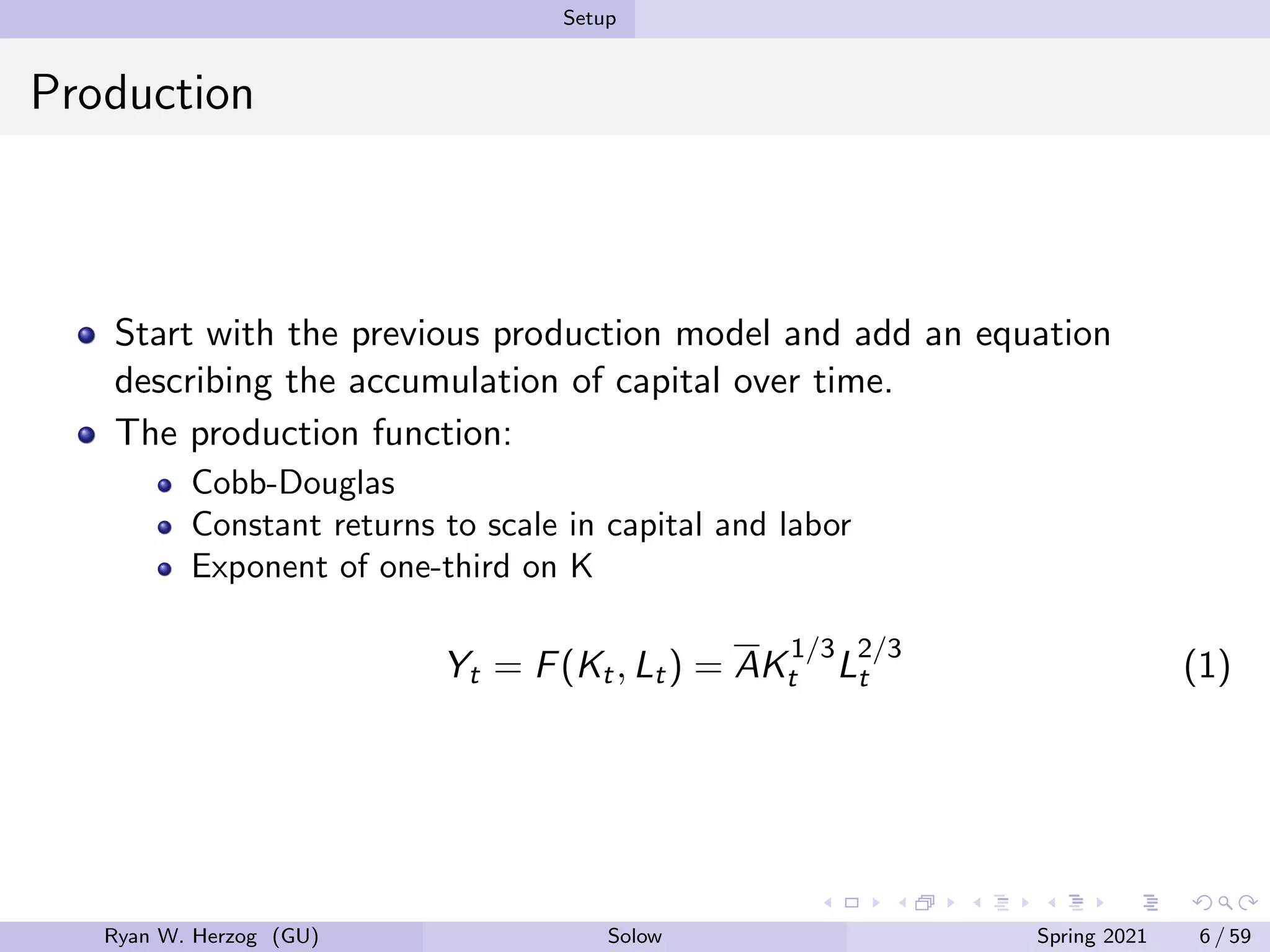
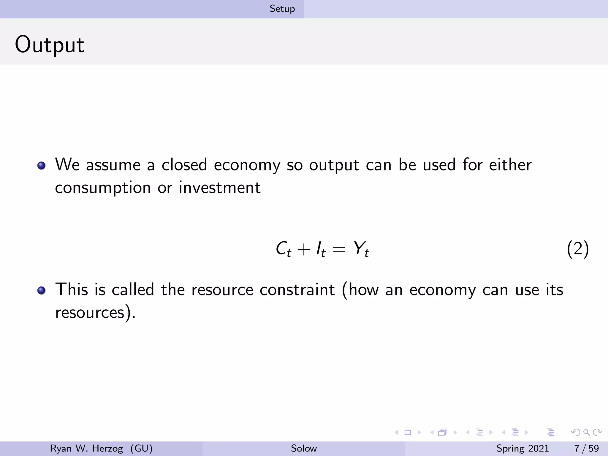
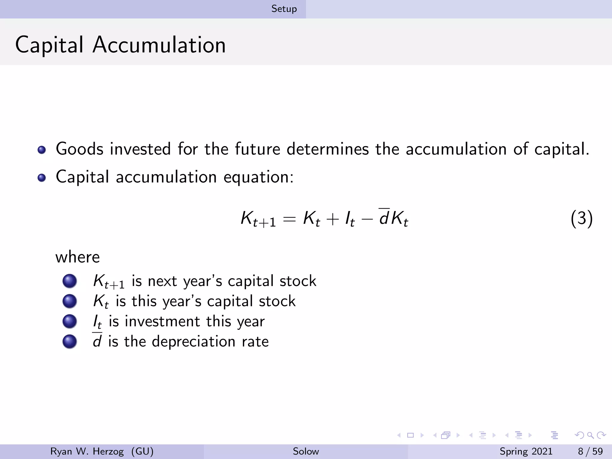
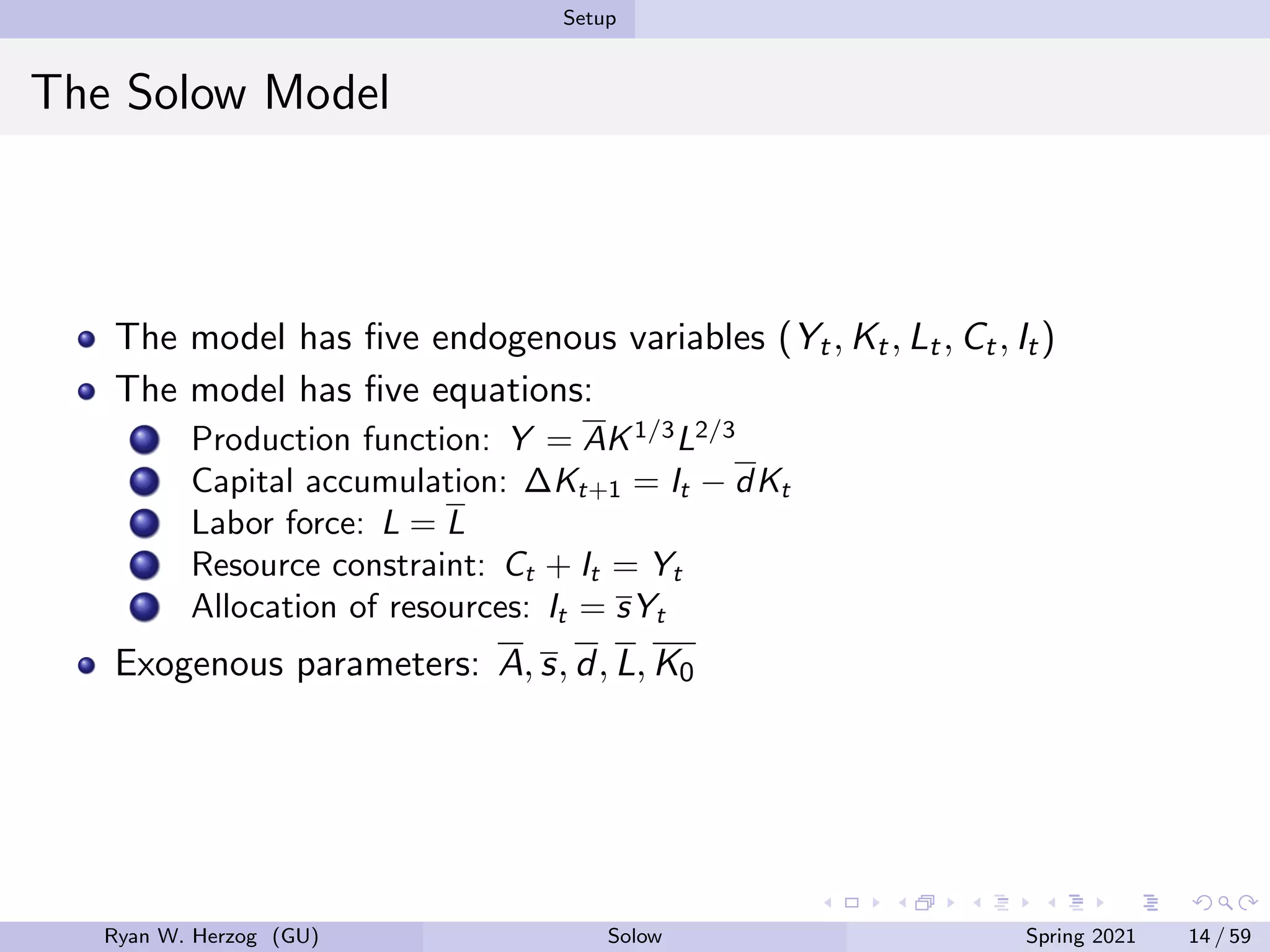

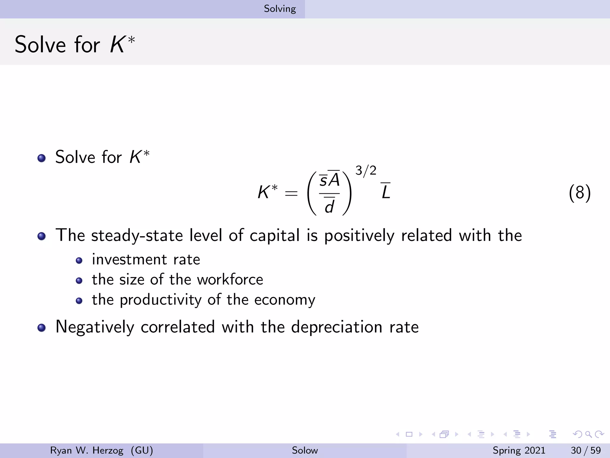
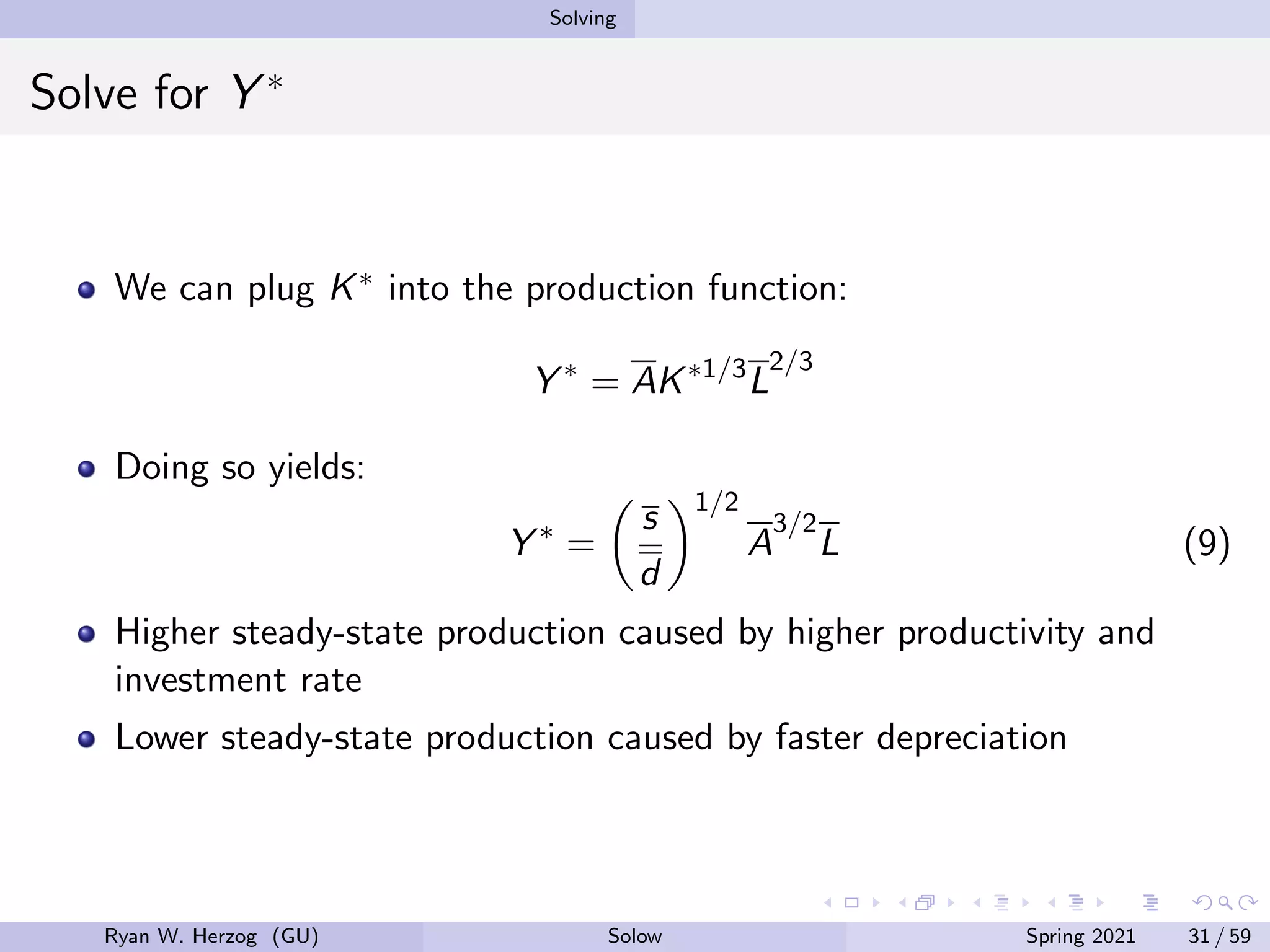
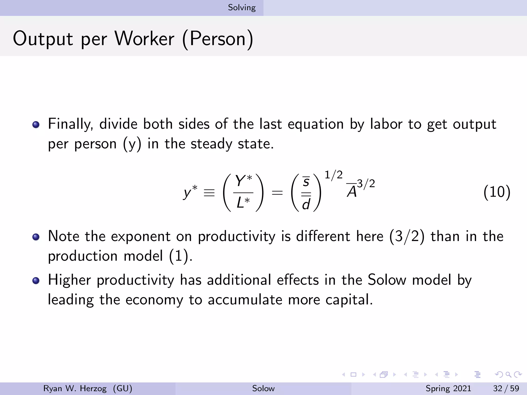


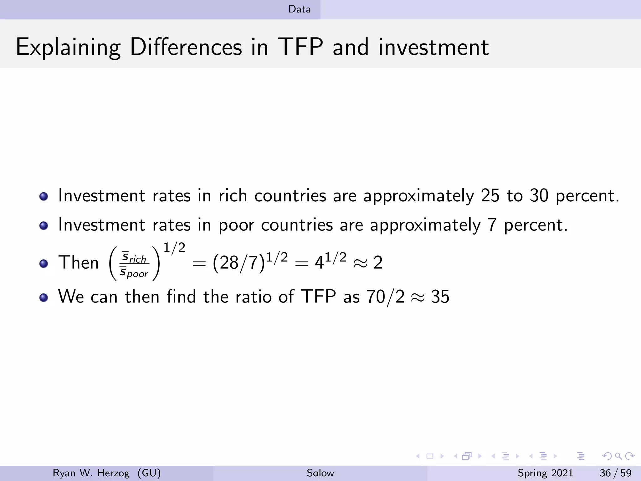
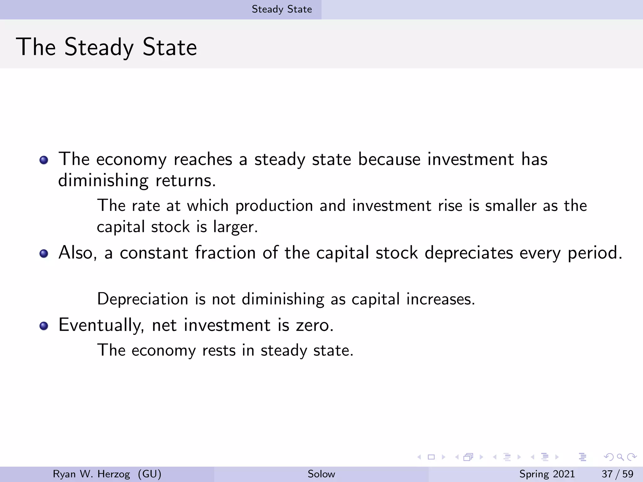
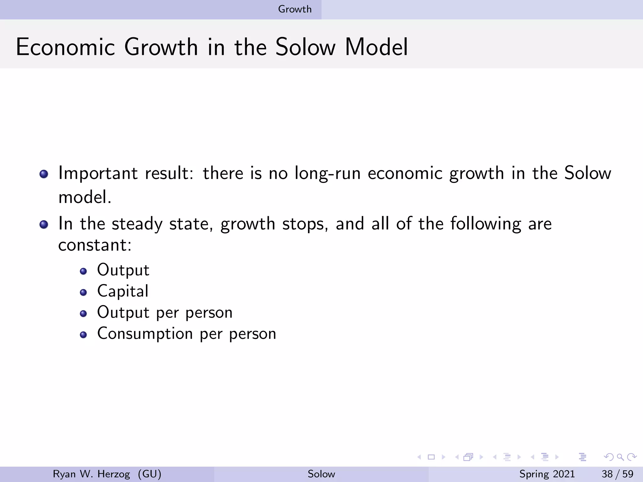
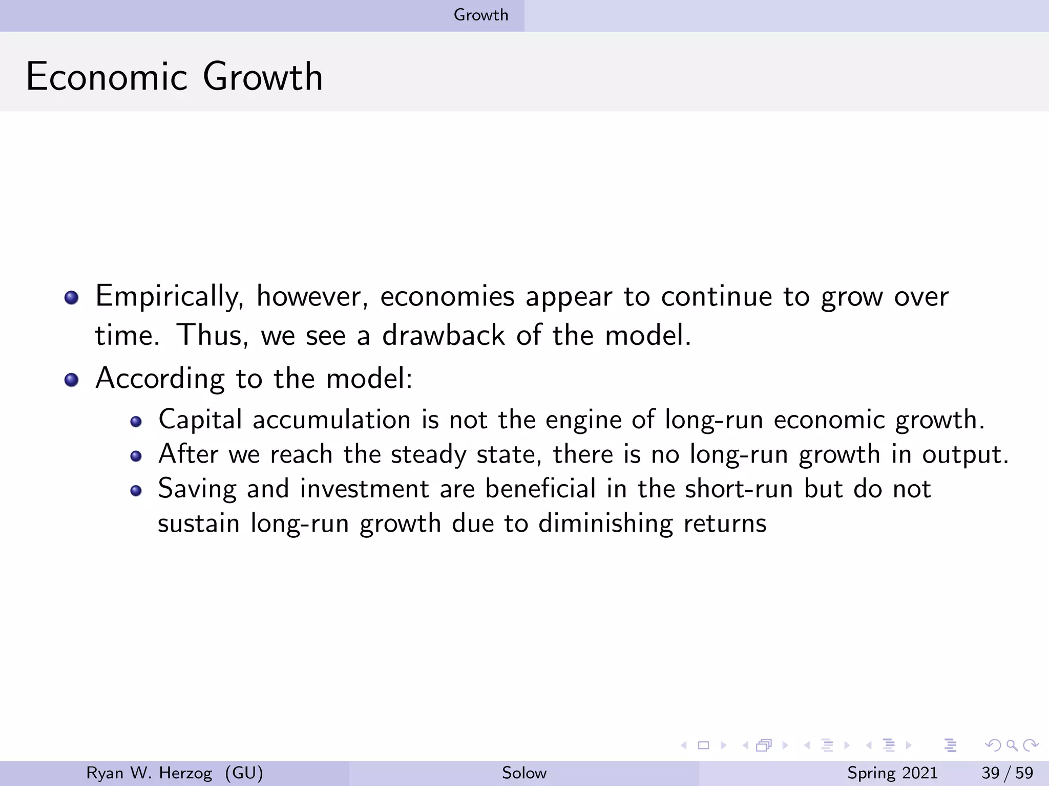


The document provides an overview of the Solow growth model, which models economic growth through capital accumulation over time. It describes the key components of the model, including the production function, capital accumulation equation, investment determination, and steady state. The model predicts that economies will eventually stop growing as they approach the steady state, due to diminishing returns to capital. However, it does not fully explain long-run economic growth. The document also discusses how the model can be used to analyze the effects of changes to parameters like the investment and depreciation rates.