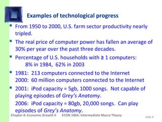
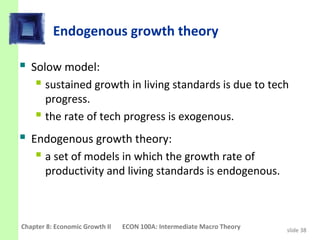
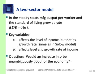
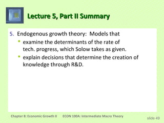
This document discusses economic growth and technological progress. It begins by introducing the Solow growth model and its limitations in accounting for long-run growth. The chapter then incorporates technological progress into the Solow model by including labor-augmenting technological change. It discusses how this affects the model's predictions and steady states. Later sections examine empirical evidence on growth, including balanced growth, conditional convergence between countries, and the roles of capital accumulation and productivity in determining income differences. The chapter concludes by considering how policies like free trade may impact productivity and long-run growth.
This document summarizes key concepts from Chapter 8 of an economics textbook on economic growth. It discusses how to incorporate technological progress into the Solow growth model by including a variable for labor efficiency that grows exogenously over time. It then reviews empirical evidence on growth, including balanced growth, conditional convergence between countries, and the relationship between factor accumulation and production efficiency. Finally, it examines policy issues such as evaluating a country's saving rate and how to increase savings and allocate investment between different types of capital.
This chapter introduces the Solow growth model, which examines how capital accumulation and population growth impact economic growth and living standards over the long run. The key aspects covered include:
- The Solow model framework of production, consumption, investment, and capital accumulation over time.
- How economies converge to a steady state level of capital per worker and output per worker.
- How factors like the saving rate can impact the steady state level and long-run growth.
- The "Golden Rule" concept of finding the optimal saving rate and capital stock that maximizes long-run consumption per person.
Policymakers debate whether monetary and fiscal policy should be active or passive in response to economic fluctuations, and whether policy should be set by rule or at the discretion of officials. Arguments for active policy include reducing economic hardship during recessions, while critics argue policies have long and variable lags. Policy rules aim to increase credibility and reduce time inconsistency problems, like central banks targeting an inflation rate or following the Taylor rule. The optimal approach remains an open debate among economists.
This document summarizes key points from a chapter about government debt. It discusses several topics:
1. The size of government debt in various countries, with Japan having the highest debt-to-GDP ratio at 159% and the U.S. at 64%.
2. Traditional and Ricardian views on the effects of government debt. The traditional view is that debt crowds out investment, while the Ricardian view is that debt has no real effects due to forward-looking consumers.
3. Problems in measuring budget deficits, such as not accounting for inflation, capital assets, or future liabilities for programs like Social Security. Correcting for these issues can significantly change deficit estimates.
This chapter introduces the concepts of the business cycle, aggregate demand, aggregate supply, and the model of aggregate demand and aggregate supply. It discusses how the economy behaves differently in the short-run versus long-run. In the short-run, many prices are sticky so the aggregate supply curve is horizontal, but in the long-run prices are flexible so the aggregate supply curve is vertical. The model can be used to analyze how shocks like changes in the money supply, velocity, or supply shocks impact output and inflation in both the short-run and long-run. An example is given of the 1970s oil shocks, which were adverse supply shocks that increased costs and shifted the short-run aggregate supply curve
This document provides an overview of classical macroeconomic theory. It discusses how classical economics emerged as a revolution against mercantilism, emphasizing free markets and real factors of production over money and trade balances. Key aspects of classical theory covered include:
- Labor and capital markets clear through price adjustments to equilibrium.
- Firms maximize profits by equaling marginal revenue product to factor prices.
- Production depends on labor, capital and technology. Increases in these real factors of supply are what increase output.
- Money is neutral, having no long-run impact on real variables like output and employment.
This document provides an overview of classical theories of inflation and the quantity theory of money. It defines key concepts like money, inflation, the money supply, and velocity. The quantity theory of money posits that inflation is primarily caused by increases in the money supply that outpace economic growth. It predicts a direct relationship between money growth and inflation. The document uses graphs and international data to show this relationship generally holds in practice and discusses implications for interest rates.
This document discusses multicollinearity, which occurs when explanatory variables are linearly correlated. It addresses the nature of multicollinearity, whether it is a problem, its practical consequences, how to detect it, and ways to alleviate it. In the case of perfect multicollinearity, regression coefficients are indeterminate and have infinite standard errors. With imperfect but high multicollinearity, coefficients can be estimated but have large variances, leading to wide confidence intervals and insignificant t-ratios despite a high R-squared value. Regressions also become sensitive to small data changes.
1) The chapter uses the IS-LM model to analyze the effects of fiscal and monetary policy shocks on aggregate output and the interest rate in the short run.
2) Fiscal policy like increases in government spending or tax cuts shift the IS curve right, raising output. Monetary policy like increases in the money supply shift the LM curve down, lowering interest rates and raising output.
3) Shocks like increases in wealth from a stock market boom shift the IS curve right, raising output, while shocks that increase money demand like credit card fraud shift the LM curve left, lowering output.
4) In the long run, price adjustments return output to potential as the price level falls to accommodate any short
The document discusses the Mundell-Fleming model of the open economy and exchange rate regimes. It provides an overview of the key assumptions and components of the Mundell-Fleming model, including the IS* and LM* curves. It then analyzes the effects of fiscal policy, monetary policy, and trade policy under both floating and fixed exchange rate systems. The document concludes with two case studies on financial crises in Mexico and Southeast Asia that illustrate the model.
This document provides an introduction to macroeconomics. It defines macroeconomics as the study of large-scale national economies and the policies that governments use to affect economic performance. The document then discusses key macroeconomic concepts including gross domestic product (GDP), real GDP and economic growth, issues like growth, unemployment and inflation, and comparisons of output and growth across countries. It also covers business cycles, budget deficits, international trade, and differences in economic perspectives.
This document provides an overview of macroeconomic theory regarding short-term fluctuations in output and employment (i.e. the business cycle) using aggregate demand/aggregate supply models. It explains that in the short-run, prices are sticky but flexible in the long-run, leading to different aggregate supply curves (SRAS, LRAS). The AD/AS framework is used to analyze how demand and supply shocks can cause fluctuations and how stabilization policy aims to minimize changes in output and employment.
policy implication of the classical Equilibrium modelShahidMunir33
The document discusses the effects of reducing income taxes according to the classical equilibrium model. It states that reducing income taxes would:
1) Increase disposable income, leading to higher consumption and aggregate demand. Interest rates may also increase as the government issues bonds to replace lost revenue.
2) Increase the real wages of individuals by reducing the percentage of income paid in taxes. This would shift the aggregate labor supply curve to the right, increasing employment and overall output.
3) Shift the aggregate supply curve to the right as well, which would decrease price levels according to the new general equilibrium of the model.
Monetarism is an economic school of thought that stresses the primary importance of the money supply in determining nominal GDP and price levels. It challenges Keynesian economics by arguing that monetary policy, not fiscal policy, should be used to stabilize the economy. Monetarists believe the central bank should target money supply growth and follow fixed rules, rather than have discretion, as monetary factors are more important than fiscal interventions in impacting economic outcomes.
The document provides an overview of monetarism and Milton Friedman's restatement of the quantity theory of money. It discusses four key aspects of monetarism: (1) that fluctuations in the money supply are the dominant cause of fluctuations in real output; (2) monetarism's use of an expectations-augmented Phillips curve; (3) a monetary approach to exchange rates; and (4) support for monetary policy rules over discretionary policies. It also summarizes Friedman's restatement of the quantity theory and three arguments for adopting a rule-based monetary policy of steady money supply growth.
New Keynesian economics evolved in response to new classical critiques of Keynesian macroeconomics. It incorporates Keynesian ideas like sticky prices and wages to explain short-run economic fluctuations. A key difference from new classical economics is the assumption that prices and wages adjust slowly rather than quickly clearing markets. This allows for involuntary unemployment and a role for monetary policy. A new synthesis has emerged merging tools from both new classical and new Keynesian models.
Here are the key impacts of an increase in investment demand in a small open economy:
- Investment demand I(r*) increases.
- Saving S does not change.
- Net capital outflow decreases as domestic investment increases and saving remains the same.
- Net exports NX decrease as the trade balance deteriorates to finance the higher investment through net capital inflows.
So in summary, an increase in investment demand leads to a deterioration in the trade balance (lower NX) and lower net capital outflow, while saving remains unchanged.
CHAPTER 5 The Open Economy slide 23
1. The document discusses the IS-LM model and how it can be used to analyze the effects of fiscal and monetary policy. It presents the IS and LM curves and how they represent equilibrium in the goods and money markets.
2. Fiscal policy like increases in government spending can shift the IS curve right, raising output and interest rates. Monetary policy like increases in the money supply can shift the LM curve down, lowering interest rates and raising output.
3. Shocks to aggregate demand are analyzed using the IS-LM model, and the model can also show the transition from short-run to long-run equilibrium when prices adjust over time.
This document provides an overview of several prominent theories of consumption, including:
1) John Maynard Keynes' theory that current consumption depends on current income. Later theories found problems with Keynes' prediction that consumption would grow more slowly than income over time.
2) Irving Fisher's intertemporal choice theory, which assumes consumers maximize lifetime satisfaction subject to an intertemporal budget constraint. This theory formed the basis for later work on consumption.
3) Franco Modigliani's life-cycle hypothesis, which proposes consumption depends on lifetime resources and income varies systematically over a consumer's life cycle, allowing saving to achieve smooth consumption. This theory helped solve the "consumption puzzle."
4)
The document discusses technological progress in economic growth models. It introduces an endogenous growth model where the rate of technological progress is determined within the model rather than assumed constant. It also discusses policies that can promote economic growth, such as increasing the savings rate, allocating investment efficiently among different types of capital, and encouraging innovation. Empirical evidence generally confirms predictions of the Solow growth model.
1) There are four phases of the business cycle: recession, depression, peak, and trough. Recessions are periods of economic contraction while expansions include booms.
2) Business cycles cause fluctuations in real GDP and cyclical unemployment. The size of recessions and expansions can be measured by comparing actual output and unemployment to potential output and the natural rate of unemployment.
3) Short-term economic fluctuations are primarily caused by changes in aggregate spending as prices adjust and markets reach equilibrium. Policymakers aim to stabilize the economy by closing output gaps between actual and potential output.
This chapter discusses recent advances in business cycle theory, including Real Business Cycle theory and New Keynesian economics. Real Business Cycle theory assumes flexible prices and that fluctuations result from optimal responses to productivity shocks, while New Keynesian economics focuses on explaining price stickiness through microeconomic factors like menu costs. There is ongoing debate around the assumptions and empirical evidence regarding both approaches.
This document summarizes key concepts from Chapter 12 of Mankiw's Macroeconomics textbook on open economy macroeconomics. It introduces the Mundell-Fleming model, which uses the IS-LM framework to analyze the effects of fiscal and monetary policy in a small open economy. It discusses the implications of floating versus fixed exchange rates and how this determines the effectiveness of different policies. It also examines the impacts of interest rate differentials and trade policies. The summary slides provide a concise overview of the model and the main policy conclusions.
Domar's growth model from 1946 analyzes how a capitalist economy can grow at a constant rate after reaching full employment. It assumes aggregate supply equals aggregate demand during steady growth. The model shows that for steady growth, the rates of investment, capital stock growth, output growth, and employment growth must all be equal. It derives the equation that the growth rate equals the savings ratio multiplied by the incremental output-capital ratio. Investment has dual effects of increasing both aggregate demand and productive capacity in the long-run.
This document provides an overview of the Solow growth model, which examines how economic growth and standards of living are determined in the long run. It introduces key concepts such as the production function, saving rate, depreciation rate, capital accumulation, and steady state. The steady state is the level of capital where investment just offsets depreciation and capital remains constant. The model predicts that countries with higher saving and investment rates will have higher levels of capital and income per worker in the long run. It also discusses finding the optimal saving rate and capital stock, known as the Golden Rule, which maximizes consumption.
The document discusses government debt and perspectives on it. It covers measurement problems with the deficit figure due to inflation, business cycles, and uncounted liabilities. It also summarizes the traditional view that debt lowers national saving versus the Ricardian view that it does not affect saving. Most economists oppose a balanced budget rule as it hinders fiscal policy goals like stabilization.
Patinkin argues that the classical dichotomy between real and monetary sectors is invalid. When the money supply changes, it affects relative prices through the real balance effect. Specifically:
1) If money supply increases, prices rise proportionally. This reduces the real value of cash balances and lowers demand for goods, putting downward pressure on prices.
2) The real balance effect restores equilibrium by linking demand for goods and money - if prices fall, real balances and demand for goods rise, putting upward pressure back on prices.
3) Therefore, changes in the money supply can change the price level without affecting relative prices, reconciling monetary and real factors and invalidating the dichotomy between the two.
The neoclassical theory of interest, or loanable funds theory, holds that the interest rate is determined by the supply and demand for loanable funds. The demand for loanable funds comes from investment, consumption/dissaving, and hoarding. The supply comes from savings, bank credit, dishoarding, and disinvestment. The interest rate reaches equilibrium when the total demand for loanable funds equals the total supply. Critics argue the theory assumes full employment, does not precisely determine the interest rate, and is impractical.
The document discusses economic growth models including the Harrod-Domar growth model. It presents the key assumptions and equations of the Harrod-Domar model, which links the growth rate to the savings rate and capital-output ratio. However, the document notes that the Harrod-Domar model treats factors like the savings rate and population growth rate as constant, when in reality they may change as the economy grows, making them endogenous rather than exogenous variables.
This document provides an overview of macroeconomic concepts including national accounts, growth accounting, and the Solow growth model. It discusses how factors like technology, capital stock, and labor force contribute to economic growth. The Solow growth model assumes steady state growth and constant returns to scale. In steady state, the capital-labor ratio remains constant and savings must equal investment. The document also shares a quote from Beatriz Orresta about her family struggling to afford food due to declining incomes during difficult economic times.
This document provides an overview of the history of labor unions in the United States from the early 19th century through the mid-20th century. It discusses early union development being stunted until the 1930s due to widespread anti-union sentiment among Americans and employers. The document then covers key events that shaped the labor movement such as violent strikes in the 1870s-1890s, the rise of national unions in the late 19th century, and pro-union legislation passed during the Great Depression in response to widespread economic hardship.
1. The document discusses economic growth accounting and theories of economic growth.
2. Growth accounting explains that economic growth is due to increases in inputs like capital and labor as well as productivity increases from technological progress. The neoclassical growth model predicts economies will reach a steady state of constant per capita output and capital.
3. The document also examines factors that influence differences in economic growth rates between countries, such as capital accumulation, population growth, human capital development, and natural resources. It analyzes growth empirically and discusses implications of growth theory.
The document discusses the history and development of labor unions in the United States from the colonial period through modern times. It covers key events and legislation that impacted unions such as the Great Depression, World War II, the Taft-Hartley Act. The document also examines topics related to employment, wages, gender pay differences, and minimum wage.
World Press Photo 10 was an exhibition held from May 28, 2010 at the Shihlin Paper Corporation in Taiwan. The exhibition featured award-winning press photographs from around the world in 2010 that were selected by the World Press Photo Foundation.
This presentation exhibits the journey of Pakistan economy. The historical performance is exhibited and explained through contemporary theories of economics
Labor unions first emerged in the United States in the late 18th century as organizations that banded together workers for mutual aid and protection against poor working conditions and low pay. Key figures in the early labor movement fought for the rights of industrial and agricultural workers. Unions continue to influence politics and advocate for workers' interests today, though membership has declined. Events like Labor Day still honor the past contributions of the American labor movement.
This document contains slides from a chapter on economic growth from a macroeconomics textbook. It introduces the Solow growth model, which examines how a closed economy's saving rate and population growth affect its long-run standard of living and capital stock. The model shows diminishing returns to capital as capital per worker increases. It defines concepts like the steady state, where investment just offsets depreciation, keeping the capital stock constant. Numerical examples demonstrate how the capital stock approaches the steady state over time as investment exceeds depreciation when capital is below the steady state level.
The Harrod-Domar growth model uses 3 key variables to determine the growth rate:
1. The saving rate, which determines how much can be invested.
2. Capital productivity, or how much output increases with each unit of new capital.
3. The depreciation rate, which accounts for aging of the existing capital stock.
The model's formula is: Growth Rate = Saving Rate x Capital Productivity - Depreciation Rate. It provides a simple framework for analyzing how changes to these variables impact long-term economic growth.
The Solow Growth Model describes a pure production economy where population grows at a constant rate, consumers save a fixed portion of income, and firms produce output according to a Cobb-Douglas production function. The model shows that the per capita capital stock reaches a steady state where the marginal product of capital equals the capital depreciation rate plus population growth rate, divided by the savings rate. The document provides an example comparing the steady state capital stock under different population growth rates and savings rates.
Schumpeterian theory views economic development as resulting from "new combinations" introduced through innovations. These innovations disrupt equilibrium and are introduced by entrepreneurs seeking profits. Entrepreneurs are financed through bank credit expansion, fueling investment and economic growth. However, this leads to a boom-bust cycle as old industries are displaced. Over time, capitalism decays due to weakening entrepreneurship, family institutions, and property rights, transitioning toward socialism. Critics argue Schumpeter overstates the role of idealized innovators and the cyclical nature of innovation-driven changes.
This document summarizes key aspects of the Solow growth model and endogenous growth theory. It discusses how technological progress is incorporated in the Solow model and its effects on variables like output per worker. It also examines empirical evidence about balanced growth and the relationship between factor prices and productivity in the US. The document analyzes the US saving rate using the Solow model and considers the impacts of different public policies on economic growth. Finally, it introduces endogenous growth theory and how it rejects the exogenous technological progress assumption of the Solow model.
The document summarizes key concepts from an intermediate macroeconomics textbook chapter on long-run economic growth. It introduces growth accounting and examines the neoclassical and endogenous growth models. The neoclassical model shows output growing at the population rate unless productivity increases. The endogenous model explains productivity growth endogenously through constant or increasing returns to capital. Government policies that boost savings/investment or productivity can increase long-run growth rates.
The document summarizes key growth models:
1) The Harrod-Domar model assumes fixed capital-output and capital-labor ratios and that the growth rate is determined by the savings ratio. However, it fails to account for substitutability between factors.
2) The Solow-Swan model introduces variable factor ratios and exogenous technological progress. It shows how capital accumulation, labor force growth, and technology affect output over time.
3) Endogenous growth models developed by Romer relax the assumption of diminishing returns to capital and allow technological progress to be endogenous.
The document summarizes key concepts from macroeconomic growth models including the Harrod-Domar, Solow-Swan, and endogenous growth models. It discusses the Harrod-Domar model which relates an economy's growth rate to its capital stock and savings ratio. It then summarizes the Solow-Swan model which incorporates technological progress and assumes diminishing returns to capital. The model predicts economies will eventually reach a steady state level of capital and output. Finally, it briefly mentions endogenous growth models which seek to explain technological progress.
1) The document summarizes key aspects of the Solow growth model, including how capital accumulation, depreciation, investment, and population growth determine an economy's steady state level of output.
2) It shows graphically how the steady state is reached through the balance of investment and depreciation, and how population growth lowers the steady state.
3) The "Golden Rule level of capital" is defined as the steady state that maximizes consumption, where the marginal product of capital equals the depreciation rate.
This document provides an overview of key concepts from Chapter Seven of the textbook Macroeconomics by N. Gregory Mankiw. It discusses the Solow growth model and how it treats capital accumulation. It then explains how population growth and technological progress can be incorporated into the model. The summary concludes by noting that the Solow model predicts balanced growth and convergence between economies in the long run.
This document provides an overview of Chapter 3 from a macroeconomics textbook. It covers:
1) The determination of GDP based on the fixed supplies of capital and labor and the production function.
2) How factor prices (wages and rental rates) are determined by supply and demand in factor markets.
3) How total income is distributed to labor and capital income based on factor payments.
4) The components of aggregate demand - consumption, investment, government spending - and how their interaction determines equilibrium in the goods market.
1. The document provides an overview of the Solow growth model, which shows how capital accumulation, labor force growth, and technological advances interact in an economy and affect total output.
2. It examines how the model treats the accumulation of capital over time and how savings, depreciation, population growth, and technological progress influence the long-run capital stock and output.
3. The model predicts that economies with higher savings rates or population growth rates will reach different steady-state levels of capital and output per worker.
This chapter discusses the determination of national income and its distribution in a closed economy. It introduces the production function and factors of production, capital and labor. It explains that total output is determined by factor supplies and technology. Factor prices, the wage rate and rental rate, are determined by supply and demand in factor markets. Total income is distributed to factors based on their marginal products. The chapter then covers the components of aggregate demand - consumption, investment, and government spending. It presents the loanable funds market model to show how interest rates adjust to equilibrate saving and investment.
This document discusses the Solow growth model and economic convergence. It introduces key equations of the Solow model relating capital per worker (k), GDP per worker (y), saving rate (s), depreciation rate (δ), and population growth rate (n). It explains that economies starting at different levels of capital per worker will converge over time towards the same steady-state level as the lower starting economy grows faster initially. GDP per worker convergence follows from capital per worker convergence. Conditional and absolute convergence are defined.
1) The document summarizes key concepts from Chapter 3 of a macroeconomics textbook, including how total national income is determined by aggregate supply and demand.
2) It explains how factor prices like wages and rental rates are determined by supply and demand in factor markets and how this determines the distribution of total income.
3) It outlines the components of aggregate demand - consumption, investment, and government spending - and how their interaction with aggregate supply determines equilibrium in the goods market and the loanable funds market.
This document provides an overview of key macroeconomic statistics including Gross Domestic Product (GDP), the Consumer Price Index (CPI), and the unemployment rate. It discusses how GDP can be measured through expenditures, income, and value added. The components of GDP expenditures are defined as consumption, investment, government spending, and net exports. Real GDP is introduced to control for inflation. The GDP deflator and inflation rates are also explained.
The document summarizes the Solow growth model of macroeconomics. It explains that the model focuses on long-run economic growth driven by capital accumulation from savings and investment. While higher savings can increase growth in the short-run, in the long-run the economy reaches a steady-state where population growth determines the rate of growth and savings only impacts output levels, not growth rates. The model uses mathematical equations to represent capital accumulation and its impact on output over time.
This document discusses endogenous growth theory and compares it to the neoclassical growth model. It summarizes two core endogenous growth models: the AK model and a "learning by doing" model. The AK model endogenizes long-run growth by having output be a linear function of capital alone. This causes savings rates to permanently impact the growth rate. The "learning by doing" model features knowledge spillovers that increase productivity based on average capital levels. Both models generate sustained long-run growth, unlike the neoclassical model. The document then discusses how international capital market integration can further boost growth by allowing more efficient global allocation of capital.
The document provides an overview of the IS-LM model of aggregate demand. It explains that the IS curve models the goods market relationship between interest rates and income, while the LM curve models the money market relationship between interest rates and income. It also discusses the Keynesian cross diagram and how it can be used to analyze how changes in fiscal policy like government purchases or taxes will affect equilibrium income levels through multiplier effects. The document concludes by explaining that the intersection of the IS and LM curves determines the aggregate demand equilibrium for a given price level.
The document presents a New Keynesian model with a small open economy. It introduces the model, which includes Calvo staggered prices, perfect international financial markets, PPP in the long run, and identical preferences across countries. The model derives a two-equation system for inflation and output gaps, as well as characterizes monetary policy. It then calibrates the model under technology and cost-push shocks for closed, slightly open, and moderately open economies.
This document discusses differences in living standards and economic growth rates around the world. It begins by showing data on GDP per capita and other indicators for families in the UK, Mexico, and Mali to illustrate vast differences in living standards globally. Tables then show data on GDP per capita and growth rates for various countries from 1960-2005, demonstrating both differences in incomes and variation in growth rates. The document poses questions about why some countries are richer and grow faster than others and what policies may help raise growth rates and living standards. It then discusses various determinants of productivity that influence economic growth and living standards.
This document provides an overview of key concepts in international macroeconomics and the open economy model. It introduces accounting identities that apply to an open economy, where spending does not necessarily equal output and saving does not necessarily equal investment due to trade flows. It then presents the small open economy model, where the domestic economy is too small to affect global interest rates. In this model, the trade balance and exchange rate are determined by the interaction of domestic saving and investment with the exogenous world interest rate. Fiscal and monetary policies can influence the trade balance and exchange rate through their impact on saving and investment.
LO1. Explain how sticky prices relate to the AE model.
LO2. Explain how an economy’s investment schedule is derived from the investment demand curve & an interest rate.
LO3. The table shows different levels of output and the corresponding levels of consumption, investment, exports and aggregate expenditures to determine the equilibrium level of output where aggregate expenditures equals output.
LO4. Equilibrium is also characterized by savings equaling investment and consumption being less than output due to savings being a leakage from the circular flow of spending.
1. The document discusses using the IS-LM model to analyze the effects of shocks, fiscal policy, and monetary policy. It provides examples of analyzing different policy changes using the IS-LM diagram.
2. It then discusses how the IS-LM model can be used to derive the aggregate demand curve and analyze short-run and long-run effects of shocks. Price level adjustments move the economy from short-run to long-run equilibrium.
3. The document contains an example analyzing the 2001 US recession using the IS-LM framework, examining the effects of stock market decline, 9/11, accounting scandals, and fiscal and monetary policy responses.
This chapter introduces key concepts in macroeconomics including:
1. Facts about the business cycle such as GDP growth averaging 3-3.5% per year with large short-run fluctuations and unemployment rising during recessions.
2. The model of aggregate demand and aggregate supply which shows how the price level and output are determined in the short-run and long-run.
3. How shocks such as changes in money supply, oil prices, or velocity can temporarily push the economy away from full employment and affect inflation and output. Stabilization policies like monetary policy can be used to counteract shocks.
The document discusses how the banking system creates money through fractional-reserve banking. It provides examples showing how an initial deposit of $1000 can expand the money supply to $5000 through a series of loans and deposits across multiple banks. While banks create money, they do not create wealth, as the new money is offset by an equal amount of new debt. The Federal Reserve uses three main tools to control the money supply - open market operations, reserve requirements, and the discount rate - but cannot precisely control it as households and banks can impact the money multiplier.
This document provides an overview of key concepts from a chapter on aggregate supply and the short-run tradeoff between inflation and unemployment. It discusses three models of aggregate supply (sticky-wage, imperfect-information, sticky-price) that imply a positive relationship between output and the price level in the short run. It also covers the Phillips curve relationship between inflation and unemployment and how aggregate supply shifts over time as expectations change.
This chapter discusses macroeconomic concepts including national income, GDP, and the factors that determine and distribute total income in an economy. It presents models for how prices of labor and capital are determined by supply and demand in factor markets, and how total income is distributed to labor income and capital income based on marginal productivity. The chapter also examines the components of aggregate demand, including consumption, investment, and government spending, and how equilibrium is reached in the goods and loanable funds markets through price adjustments.
1) The chapter introduces managerial finance and describes its relationship to economics and accounting. It defines finance and outlines the major areas including financial services and managerial finance.
2) It explains the key functions of the financial manager including maximizing shareholder wealth and outlines the goals and responsibilities of corporate governance.
3) It differentiates between individual and institutional investors and their roles in corporate governance.
1. 8
C H A P T E
R
Economic Growth II:
Technology, Empirics, and Policy
8-1 Technological Progress in the Solow Model
8-2 From Growth Theory to Growth Empirics
8-3 Policies to Promote Growth
8-4 Endogenous Growth Theory
2. In this chapter, you will learn…
how to incorporate technological progress in the
Solow model
about policies to promote growth
about growth empirics: confronting the theory with
facts
two simple models in which the rate of technological
progress is endogenous
Chapter 8: Economic Growth II ECON 100A: Intermediate Macro Theory slide 2
3. Introduction
In the Solow model of Chapter 7,
the production technology is held constant.
income per capita is constant in the steady state.
Neither point is true in the real world:
1904-2004: U.S. real GDP per person grew by a factor
of 7.6, or 2% per year.
examples of technological progress abound
(see next slide).
Chapter 8: Economic Growth II ECON 100A: Intermediate Macro Theory slide 3
4. Examples of technological progress
From 1950 to 2000, U.S. farm sector productivity nearly
tripled.
The real price of computer power has fallen an average of
30% per year over the past three decades.
Percentage of U.S. households with ≥ 1 computers:
8% in 1984, 62% in 2003
1981: 213 computers connected to the Internet
2000: 60 million computers connected to the Internet
2001: iPod capacity = 5gb, 1000 songs. Not capable of
playing episodes of Grey’s Anatomy.
2006: iPod capacity = 80gb, 20,000 songs. Can play
episodes of Grey’s Anatomy.
Chapter 8: Economic Growth II ECON 100A: Intermediate Macro Theory slide 4
5. Technological progress in the Solow
model
A new variable: E = labor efficiency
Assume:
Technological progress is labor-augmenting:
it increases labor efficiency at the exogenous rate g:
∆E
g =
E
Chapter 8: Economic Growth II ECON 100A: Intermediate Macro Theory slide 5
6. Technological progress in the Solow
model
We now write the production function as:
Y = F (K , L ×E )
where L × E = the number of effective
workers.
Increases in labor efficiency have the
same effect on output as increases in
the labor force.
Chapter 8: Economic Growth II ECON 100A: Intermediate Macro Theory slide 6
7. Technological progress in the Solow
model
Notation:
y = Y/LE = output per effective worker
k = K/LE = capital per effective worker
Production function per effective worker:
y = f(k)
Saving and investment per effective worker:
s y = s f(k)
Chapter 8: Economic Growth II ECON 100A: Intermediate Macro Theory slide 7
8. Technological progress in the Solow
model
(δ + n + g)k = break-even investment:
the amount of investment necessary
to keep k constant.
Consists of:
δ k to replace depreciating capital
n k to provide capital for new workers
g k to provide capital for the new “effective”
workers created by technological progress
Chapter 8: Economic Growth II ECON 100A: Intermediate Macro Theory slide 8
9. Technological progress in the Solow
model
Investment, ∆ k = s f(k) − (δ +n +g )k
break-even
investment
( δ +n + g ) k
sf(k)
k* Capital per
Chapter 8: Economic Growth II worker, k
ECON 100A: Intermediate Macro slide 9
Theory
10. Steady-state growth rates in the
Solow model with tech. progress
Steady-state
Variable Symbol
growth rate
Capital per
k = K/(L×E ) 0
effective worker
Output per
y = Y/(L×E ) 0
effective worker
Output per worker (Y/ L) = y×E g
Total output Y = y×E×L n+g
Chapter 8: Economic Growth II ECON 100A: Intermediate Macro slide 10
Theory
11. The Golden Rule
To find the Golden Rule capital stock,
express c* in terms of k*:
In the Golden
In the Golden
c = y
* *
− i *
Rule steady state,
Rule steady state,
= f (k* ) − (δ + n + g) k* the marginal
the marginal
product of capital
product of capital
c* is maximized when net of depreciation
net of depreciation
MPK = δ + n + g equals the
equals the
pop. growth rate
pop. growth rate
or equivalently, plus the rate of
plus the rate of
MPK − δ = n + g tech progress.
tech progress.
Chapter 8: Economic Growth II ECON 100A: Intermediate Macro Theory slide 11
12. Growth empirics:
Balanced growth
Solow model’s steady state exhibits
balanced growth - many variables grow
at the same rate.
Solow model predicts Y/L and K/L grow at the same
rate (g), so K/Y should be constant.
This is true in the real world.
Solow model predicts real wage grows at same rate
as Y/L, while real rental price is constant.
This is also true in the real world.
Chapter 8: Economic Growth II ECON 100A: Intermediate Macro Theory slide 12
13. Growth empirics: Convergence
Solow model predicts that, other things equal, “poor”
countries (with lower Y/L and K/L) should grow faster
than “rich” ones.
If true, then the income gap between rich & poor
countries would shrink over time, causing living
standards to “converge.”
In real world, many poor countries do NOT grow faster
than rich ones. Does this mean the Solow model fails?
Chapter 8: Economic Growth II ECON 100A: Intermediate Macro Theory slide 13
14. Growth Empirics: Convergence
Solow model predicts that, other things equal, “poor”
countries (with lower Y/L and K/L) should grow faster
than “rich” ones.
No, because “other things” aren’t equal.
In samples of countries with
similar savings & pop. growth rates,
income gaps shrink about 2% per year.
In larger samples, after controlling for differences in
saving, pop. growth, and human capital, incomes
converge by about 2% per year.
Chapter 8: Economic Growth II ECON 100A: Intermediate Macro Theory slide 14
15. Growth empirics: Convergence
What the Solow model really predicts is
conditional convergence - countries converge
to their own steady states, which are determined by
saving, population growth, and education.
This prediction comes true in the real world.
Chapter 8: Economic Growth II ECON 100A: Intermediate Macro Theory slide 15
16. Growth empirics: Factor accumulation vs.
production efficiency
Differences in income per capita among countries can
be due to differences in
1. capital – physical or human – per worker
2. the efficiency of production
(the height of the production function)
Studies:
both factors are important.
the two factors are correlated: countries with higher
physical or human capital per worker also tend to
have higher production efficiency.
Chapter 8: Economic Growth II ECON 100A: Intermediate Macro Theory slide 16
17. Growth empirics: Factor accumulation vs.
production efficiency
Possible explanations for the correlation between
capital per worker and production efficiency:
Production efficiency encourages capital
accumulation.
Capital accumulation has externalities that raise
efficiency.
A third, unknown variable causes
capital accumulation and efficiency to be higher in
some countries than others.
Chapter 8: Economic Growth II ECON 100A: Intermediate Macro Theory slide 17
18. Growth empirics:
Production efficiency and free trade
Since Adam Smith, economists have argued that free
trade can increase production efficiency and living
standards.
Research by Sachs & Warner:
Average annual growth rates, 1970-89
open closed
developed nations 2.3% 0.7%
developing nations 4.5% 0.7%
Chapter 8: Economic Growth II ECON 100A: Intermediate Macro Theory slide 18
19. Growth empirics:
Production efficiency and free trade
To determine causation, Frankel and Romer exploit
geographic differences among countries:
Some nations trade less because they are farther
from other nations, or landlocked.
Such geographical differences are correlated with
trade but not with other determinants of income.
Hence, they can be used to isolate the impact of trade
on income.
Findings: increasing trade/GDP by 2% causes GDP per
capita to rise 1%, other things equal.
Chapter 8: Economic Growth II ECON 100A: Intermediate Macro Theory slide 19
20. Policy issues
Are we saving enough? Too much?
What policies might change the saving rate?
How should we allocate our investment between
privately owned physical capital, public infrastructure,
and “human capital”?
How do a country’s institutions affect production
efficiency and capital accumulation?
What policies might encourage faster technological
progress?
Chapter 8: Economic Growth II ECON 100A: Intermediate Macro Theory slide 20
21. Policy issues:
Evaluating the rate of saving
Use the Golden Rule to determine whether
the U.S. saving rate and capital stock are too high,
too low, or about right.
If (MPK − δ ) > (n + g ),
U.S. is below the Golden Rule steady state
and should increase s.
If (MPK − δ ) < (n + g ),
U.S. economy is above the Golden Rule steady state
and should reduce s.
Chapter 8: Economic Growth II ECON 100A: Intermediate Macro Theory slide 21
22. Policy issues:
Evaluating the rate of saving
To estimate (MPK − δ ), use three facts about the U.S.
economy:
1. k = 2.5 y
The capital stock is about 2.5 times one year’s GDP.
2. δ k = 0.1 y
About 10% of GDP is used to replace depreciating
capital.
3. MPK × k = 0.3 y
Capital income is about 30% of GDP.
Chapter 8: Economic Growth II ECON 100A: Intermediate Macro Theory slide 22
23. Policy issues:
Evaluating the rate of saving
1. k = 2.5 y
2. δ k = 0.1 y
3. MPK × k = 0.3 y
To determine δ , divide 2 by 1:
δk 0.1y 0.1
k
=
2.5 y
⇒ δ = = 0.04
2.5
Chapter 8: Economic Growth II ECON 100A: Intermediate Macro Theory slide 23
24. Policy issues:
Evaluating the rate of saving
1. k = 2.5 y
2. δ k = 0.1 y
3. MPK × k = 0.3 y
To determine MPK, divide 3 by 1:
MPK × k 0.3 y 0.3
k
=
2.5 y
⇒ MPK = = 0.12
2.5
Hence, MPK − δ = 0.12 − 0.04 = 0.08
Chapter 8: Economic Growth II ECON 100A: Intermediate Macro Theory slide 24
25. Policy issues:
Evaluating the rate of saving
From the last slide: MPK − δ = 0.08
U.S. real GDP grows an average of 3% per year,
so n + g = 0.03
Thus,
MPK − δ = 0.08 > 0.03 = n + g
Conclusion:
The U.S. is below the Golden Rule steady state:
Increasing the U.S. saving rate would increase
consumption per capita in the long run.
Chapter 8: Economic Growth II ECON 100A: Intermediate Macro Theory slide 25
26. Policy issues:
How to increase the saving rate
Reduce the government budget deficit
(or increase the budget surplus).
Increase incentives for private saving:
reduce capital gains tax, corporate income tax,
estate tax as they discourage saving.
replace federal income tax with a consumption tax.
expand tax incentives for IRAs (individual
retirement accounts) and other retirement savings
accounts.
Chapter 8: Economic Growth II ECON 100A: Intermediate Macro Theory slide 26
27. Policy issues:
Allocating the economy’s investment
In the Solow model, there’s one type of capital.
In the real world, there are many types,
which we can divide into three categories:
private capital stock
public infrastructure
human capital: the knowledge and skills that
workers acquire through education.
How should we allocate investment among these
types?
Chapter 8: Economic Growth II ECON 100A: Intermediate Macro Theory slide 27
28. Policy issues:
Allocating the economy’s investment
Two viewpoints:
1. Equalize tax treatment of all types of capital in all
industries, then let the market allocate investment to
the type with the highest marginal product.
2. Industrial policy:
Govt should actively encourage investment in capital
of certain types or in certain industries, because they
may have positive externalities
that private investors don’t consider.
Chapter 8: Economic Growth II ECON 100A: Intermediate Macro Theory slide 28
29. Possible problems with
industrial policy
The govt may not have the ability to “pick winners”
(choose industries with the highest return to capital or
biggest externalities).
Politics (e.g., campaign contributions) rather than
economics may influence which industries get
preferential treatment.
Chapter 8: Economic Growth II ECON 100A: Intermediate Macro Theory slide 29
30. Policy issues:
Establishing the right institutions
Creating the right institutions is important for
ensuring that resources are allocated to their best
use. Examples:
Legal institutions, to protect property rights.
Capital markets, to help financial capital flow to the
best investment projects.
A corruption-free government, to promote
competition, enforce contracts, etc.
Chapter 8: Economic Growth II ECON 100A: Intermediate Macro Theory slide 30
31. Policy issues:
Encouraging tech. progress
Patent laws:
encourage innovation by granting temporary
monopolies to inventors of new products.
Tax incentives for R&D
Grants to fund basic research at universities
Industrial policy:
encourages specific industries that are key for rapid
tech. progress
(subject to the preceding concerns).
Chapter 8: Economic Growth II ECON 100A: Intermediate Macro Theory slide 31
32. CASE STUDY:
The productivity slowdown
Growth in output per person
(percent per year)
1948-72 1972-95
Canada 2.9 1.8
France 4.3 1.6
Germany 5.7 2.0
Italy 4.9 2.3
Japan 8.2 2.6
U.K. 2.4 1.8
U.S. 2.2 1.5
Chapter 8: Economic Growth II ECON 100A: Intermediate Macro slide 32
Theory
33. Possible explanations for the
productivity slowdown
Measurement problems:
Productivity increases not fully measured.
But: Why would measurement problems
be worse after 1972 than before?
Oil prices:
Oil shocks occurred about when productivity
slowdown began.
But: Then why didn’t productivity speed up when
oil prices fell in the mid-1980s?
Chapter 8: Economic Growth II ECON 100A: Intermediate Macro Theory slide 33
34. Possible explanations for the
productivity slowdown
Worker quality:
1970s - large influx of new entrants into labor force
(baby boomers, women).
New workers tend to be less productive than
experienced workers.
The depletion of ideas:
Perhaps the slow growth of 1972-1995 is normal, and
the rapid growth during 1948-1972 is the anomaly.
Chapter 8: Economic Growth II ECON 100A: Intermediate Macro Theory slide 34
35. Which of these suspects is the culprit?
All of them are plausible,
but it’s difficult to prove
that any one of them is guilty.
Chapter 8: Economic Growth II ECON 100A: Intermediate Macro Theory slide 35
36. CASE STUDY:
I.T. and the “New Economy”
Growth in output per person
(percent per year)
1948-72 1972-95 1995-2004
Canada 2.9 1.8 2.4
France 4.3 1.6 1.7
Germany 5.7 2.0 1.2
Italy 4.9 2.3 1.5
Japan 8.2 2.6 1.2
U.K. 2.4 1.8 2.5
U.S. 2.2 1.5 2.2
Chapter 8: Economic Growth II ECON 100A: Intermediate Macro slide 36
Theory
37. CASE STUDY:
I.T. and the “New Economy”
Apparently, the computer revolution did not affect
aggregate productivity until the mid-1990s.
Two reasons:
1. Computer industry’s share of GDP much
bigger in late 1990s than earlier.
2. Takes time for firms to determine how to
utilize new technology most effectively.
The big, open question:
How long will I.T. remain an engine of growth?
Chapter 8: Economic Growth II ECON 100A: Intermediate Macro Theory slide 37
38. Endogenous growth theory
Solow model:
sustained growth in living standards is due to tech
progress.
the rate of tech progress is exogenous.
Endogenous growth theory:
a set of models in which the growth rate of
productivity and living standards is endogenous.
Chapter 8: Economic Growth II ECON 100A: Intermediate Macro Theory slide 38
39. A basic model
Production function: Y = A K
where A is the amount of output for each unit
of capital (A is exogenous & constant)
Key difference between this model & Solow:
MPK is constant here, diminishes in Solow
Investment: s Y
Depreciation: δ K
Equation of motion for total capital:
∆K = s Y − δ K
Chapter 8: Economic Growth II ECON 100A: Intermediate Macro Theory slide 39
40. A basic model
∆K = s Y − δ K
Divide through by K and use Y = A K to get:
∆Y ∆K
= = sA − δ
Y K
If s A > δ , then income will grow forever,
and investment is the “engine of growth.”
Here, the permanent growth rate depends
on s. In Solow model, it does not.
Chapter 8: Economic Growth II ECON 100A: Intermediate Macro Theory slide 40
41. Does capital have diminishing returns or
not?
Depends on definition of “capital.”
If “capital” is narrowly defined (only plant &
equipment), then yes.
Advocates of endogenous growth theory
argue that knowledge is a type of capital.
If so, then constant returns to capital is more
plausible, and this model may be a good description
of economic growth.
Chapter 8: Economic Growth II ECON 100A: Intermediate Macro Theory slide 41
42. A two-sector model
Two sectors:
manufacturing firms produce goods.
research universities produce knowledge that
increases labor efficiency in manufacturing.
u = fraction of labor in research
(u is exogenous)
Mfg prod func: Y = F [K, (1-u )E L]
Res prod func: ∆E = g (u )E
Cap accumulation: ∆K = s Y − δ K
Chapter 8: Economic Growth II ECON 100A: Intermediate Macro Theory slide 42
43. A two-sector model
In the steady state, mfg output per worker and
the standard of living grow at rate
∆E/E = g (u ).
Key variables:
s: affects the level of income, but not its
growth rate (same as in Solow model)
u: affects level and growth rate of income
Question: Would an increase in u be
unambiguously good for the economy?
Chapter 8: Economic Growth II ECON 100A: Intermediate Macro Theory slide 43
44. Facts about R&D
1. Much research is done by firms seeking profits.
2. Firms profit from research:
Patents create a stream of monopoly profits.
Extra profit from being first on the market with a new
product.
3. Innovation produces externalities that reduce the
cost of subsequent innovation.
Much of the new endogenous growth theory
attempts to incorporate these facts into models
to better understand technological progress.
Chapter 8: Economic Growth II ECON 100A: Intermediate Macro Theory slide 44
45. Is the private sector doing enough R&D?
The existence of positive externalities in the creation
of knowledge suggests that the private sector is not
doing enough R&D.
But, there is much duplication of R&D effort among
competing firms.
Estimates:
Social return to R&D ≥ 40% per year.
Thus, many believe govt should encourage R&D.
Chapter 8: Economic Growth II ECON 100A: Intermediate Macro Theory slide 45
46. Economic growth as “creative
destruction”
Schumpeter (1942) coined term “creative destruction”
to describe displacements resulting from technological
progress:
the introduction of a new product is good for
consumers, but often bad for incumbent producers,
who may be forced out of the market.
Examples:
Luddites (1811-12) destroyed machines that
displaced skilled knitting workers in England.
Walmart displaces many “mom and pop” stores.
Chapter 8: Economic Growth II ECON 100A: Intermediate Macro Theory slide 46
47. Lecture 5, Part II Summary
1. Key results from Solow model with tech progress
steady state growth rate of income per person
depends solely on the exogenous rate of tech progress
the U.S. has much less capital than the Golden Rule
steady state
2. Ways to increase the saving rate
increase public saving (reduce budget deficit)
tax incentives for private saving
Chapter 8: Economic Growth II ECON 100A: Intermediate Macro Theory
slide 47
48. Lecture 5, Part II Summary
3. Productivity slowdown & “new economy”
Early 1970s: productivity growth fell in the U.S. and
other countries.
Mid 1990s: productivity growth increased, probably
because of advances in I.T.
4. Empirical studies
Solow model explains balanced growth, conditional
convergence
Cross-country variation in living standards is
due to differences in cap. accumulation and in
production efficiency
Chapter 8: Economic Growth II ECON 100A: Intermediate Macro Theory
slide 48
49. Lecture 5, Part II Summary
5. Endogenous growth theory: Models that
examine the determinants of the rate of
tech. progress, which Solow takes as given.
explain decisions that determine the creation of
knowledge through R&D.
Chapter 8: Economic Growth II ECON 100A: Intermediate Macro Theory
slide 49
Editor's Notes
Chapter 7 had a single focus: the in-depth development of the Solow model with population growth. In contrast, Chapter 8 is a survey of many growth topics. First, the Solow model is extended to incorporate labor-augmenting technological progress at an exogenous rate. This is followed by a discussion of growth empirics, including balanced growth, convergence, and growth from factor accumulation vs. increases in efficiency. Next, policy implications are discussed. Finally, the chapter presents two very simple endogenous growth models. New material has been added in the 6 th edition: At the end of the “growth empirics” discussion, there’s a case study on the effects of free trade on economic growth. At the end of the chapter, there’s a discussion of Schumpeter’s notion of “creative destruction.” The models in this chapter are presented very concisely . If you want your students to master these models, you will need to have them do exercises and policy experiments with the models. The chapter includes some excellent Problems and Applications for this, which you can assign as homework or use in class to break up your lecture. If you are pressed for time and are considering skipping this chapter, I encourage you to at least cover section 8-1, so that your students will have learned the full Solow model with technological progress. One class period should be enough time to cover it, allowing for one or two in-class exercises if you wish. If you can spare a few more minutes, also consider section 8-3: it discusses policy implications, it’s not difficult or time-consuming, and students find it very interesting - it gives additional real-world relevance to the material in Chap 7 and in Section 8-1.
Source: data used to construct Figure 1-1, p.4, and some simple calculations.
Students are certainly aware that rapid technological progress has occurred. Yet, it’s fun to show these figures, to take stock of some specific kinds of technological progress. Sources: U.S. Census Bureau Wikipedia.org The Economist , various issues The Elusive Quest for Growth , by William Easterly The 2001 Statistical Abstract of the United States at http://www.census.gov/prod/2002pubs/01statab/stat-ab01.html USDA: http://www.ers.usda.gov/Data/AgProductivity/
If your students have trouble wrapping their heads around quantities in “per effective worker” terms, tell them not to worry: it’s not exactly intuitive, it’s merely a mathematical device to make the model tractable.
The only thing that’s new here, compared to Chapter 7, is that gk is part of break-even investment. Remember: k = K/LE, capital per effective worker. Tech progress increases the number of effective workers at rate g , which would cause capital per effective worker to fall at rate g (other things equal). Investment equal to gk would prevent this.
The equation that appears above the graph is the equation of motion modified to allow for technological progress. There are minor differences between this and the Solow model graph from Chapter 7: Here, k and y are in “per effective worker” units rather than “per worker” units. The break-even investment line is a little bit steeper: at any given value of k , more investment is needed to keep k from falling - in particular, gk is needed. Otherwise, technological progress will cause k = K/LE to fall at rate g (because E in the denominator is growing at rate g ). With this graph, we can do the same policy experiments as in Chapter 7. We can examine the effects of a change in the savings or population growth rates, and the analysis would be much the same. The main difference is that in the steady state, income per worker/capita is growing at rate g instead of being constant.
Table 8-1, p.219. Explanations: k is constant (has zero growth rate) by definition of the steady state y is constant because y = f(k) and k is constant To see why Y/L grows at rate g, note that the definition of y implies (Y/L) = yE. The growth rate of (Y/L) equals the growth rate of y plus that of E. In the steady state, y is constant while E grows at rate g. Y grows at rate g + n. To see this, note that Y = yEL = (yE) L. The growth rate of Y equals the growth rate of (yE) plus that of L. We just saw that, in the steady state, the growth rate of (yE) equals g. And we assume that L grows at rate n.
Remember: investment in the steady state, i*, equals break-even investment. If your students are comfortable with basic calculus, have them derive the condition that must be satisfied to be in the Golden Rule steady state.
Check out the third paragraph on p.221: It gives a nice contrast of the Solow model and Marxist predictions for the behavior of factor prices, comparing both models’ predictions with the data.
The two reasons on this slide are both implied by the Solow model.
This slide and the following one present material from a new case study in the 6 th edition, on pp.223-224. See note 4 on p.224 for references. Interpreting the numbers in this table: Sachs and Warner classify countries as either “open” or “closed.” Among the developed nations classified as “open,” the average annual growth rate was 2.3%. Among developed nations classified as “closed,” the growth rate was only 0.7% per year. The average growth rate for “open” developing nations was 4.5%. The average growth rate for “closed” developing countries was only 0.7%.
See note 4 on p.224 for references.
This section (this and the next couple of slides) presents a very clever and fairly simple analysis of the U.S. economy. When asked, students often have reasonable ideas of how to estimate MPK (e.g., look at stock market returns), n and g, but very few offer suggestions on how to estimate the depreciation rate: there are lots of different kinds of capital out there. Here, Mankiw presents a simple and elegant way to estimate the aggregate depreciation rate (which appears a couple of slides below). First, though, you should make sure your students know why the inequalities in the last two lines tell us whether our current steady-state is above or below the Golden Rule steady state. To see this, remember that the steady-state value of capital is inversely related to the steady state value of MPK. If we’re above the Golden Rule capital stock, then we have “too much” capital, so MPK will be smaller than in the Golden Rule steady state. If we’re below the GR capital stock, then MPK is higher than in the Golden Rule.
The three equations appear in the top part of the next slide. Therefore, if you wish, instead of showing this slide, you could just explain verbally what appears on this slide when you show the three equations on the next slide.
The actual U.S. economy has tens of thousands of different types of capital goods, all with different depreciation rates. Estimating the aggregate depreciation rate therefore might seem incomprehensibly complicated. But on this slide, we see Mankiw’s simple, clever, and elegant method of estimating the aggregate depreciation rate. Pretty neat!
Similarly, the method of estimating the aggregate MPK shown on this slide is far simpler and more elegant than somehow measuring and aggregating the returns on all different kinds of capital.
When the second bullet point displays on the screen, it might be helpful to remind students that, in the Solow model’s steady state, total output grows at rate n + g. Thus, we can estimate n + g for the U.S. simply by using the long-run average growth rate of real GDP.
If you have time available in class, you might consider asking students to brainstorm a list of policies or actions the government could take to increase the national saving rate. If you’ve been reading these annotations in the “notes” area of these slides, you’ve seen my suggestions on generating classroom discussion, and hopefully have tried them. If you haven’t, now would be a great time to try, and it’s easy: Get students into pairs (they need not change seats – students sitting together can work together). Ask them to take out a sheet of paper, and give them 3-4 minutes to see if they can come up with 3 different policies to increase saving. After the 3-4 minutes are up, ask for volunteers. Write down their responses on the board, and then compare the list that the class came up with to those appearing on this slide. Having students work in pairs BEFORE discussing in class takes class-time, but yields many benefits. All students become involved (while they are working in pairs), as opposed to only a few being involved if you immediately ask for responses w/o giving them time to think first. Many students don’t have the confidence to volunteer a response when their instructor asks for responses immediately after posing the question. However, if these students are given a few moments to think of possible answers, and if they have the chance to run it by a classmate first, then they will be FAR more likely to volunteer their responses. This leads to a higher quantity and quality of class participation.
Before showing the next slide, ask your students which of the two views is closest to their own.
This slide corresponds to new material for the 6 th edition of the textbook – see p. 229.
(Part of) Table 8-2 on p.231. “ Germany” in this table means W. Germany
Table 8-2 on p.231 Prior to 1995, “Germany” here refers to W. Germany. During the late 1990s into 2000, there was much talk in the business world of a “new economy” in which rapid productivity growth and high technology somehow nullified the standard rules and principles of economics (e.g., diminishing returns).
In the Solow model, the long-run economic growth rate equals the rate of technological progress, which is exogenous in the model. Hence, the Solow model is basically saying “all I can tell you is that growth in living standards depends on technological progress. I have no idea what drives technological progress.” Endogenous growth theory tries to explain the behavior of the rates of technological progress and/or productivity growth, rather than merely taking these rates as given.
This is an extremely simple model, yet has a powerful implication (to be developed below).
Y and K grow at the same rate because A is constant. Discussion: The return to capital is the incentive to invest. If capital exhibits diminishing returns, then the incentive to invest decreases as the economy grows. Hence, investment cannot be a source of sustained growth. However, in this model, MPK does not fall as K rises, so the incentive to invest never declines, people will always find it worthwhile to save and invest over and above depreciation, so investment becomes an engine of growth. The $64,000 question: Does capital exhibit diminishing or constant marginal returns? The answer is critical, for it determines whether investment explains sustained (i.e. steady-state) growth in productivity and living standards. See the next slide for discussion.
Before presenting this model, it might be helpful to tell students that it is an extension of something they already know - the Solow model with tech progress. There are two differences: First, a fraction of the labor force does not produce goods & services, but rather produces “knowledge” by doing research in universities. Second, the rate of tech progress is not exogenous, but rather depends on how fast the stock of knowledge grows, which in turn depends on how much labor the economy has allocated to research. If you have a few minutes of class time after presenting the model, you should consider having your students work problem #6 on p.243. Otherwise, assign it as a homework exercise. In regards to the specific elements of the model, Manufacturing production function: Just like in the Solow model with exogenous technological progress, output of manufactures depends on capital and the effective labor force employed in the mfg sector, (1-u)EL. Research production function: The “output” is increases in knowledge and labor efficiency. The “inputs” are labor and current knowledge. The function g() shows how changes in the amount of labor devoted to research affect the creation of new knowledge. All we need is for g( ) to be an increasing function. It does not matter whether a doubling of scientists causes the creation of knowledge to double, more than double, or less than double. Capital accumulation: Same as in the previous model -- net investment equals gross investment (sY) minus depreciation.
In this model, the steady state growth rate of the standard of living equals the growth rate of labor efficiency, just like in the Solow model with tech progress, covered at the beginning of this chapter. The difference here is that the rate of tech progress, g, is not exogenous: it depends on how much labor the economy has allocated to research. Answer to the question posed on the bottom of this slide: No . On one hand, higher u means faster growth. On the other hand, higher u means less labor is devoted to the production of goods & services. If we increase u , output of goods & services per capita will fall in the near term. But, with faster growth, output per capita will eventually be higher than it would have. Of course, if we increase u to its maximum possible value, 1, then no goods and services would be produced, and you’d have a bunch of starving geniuses. Which would be kind of odd, if you think about it. This tradeoff suggests that there must be some kind of “golden rule” for u , a value of u that maximizes well-being per capita in the steady state. Well, I’m clearly babbling now. Perhaps I should let you get back to your class preparations.
R&D = research and development An excellent quote on p.238 is relevant to fact #3: Isaac Newton once said “If I have seen farther than others, it is because I was standing on the shoulders of giants.”
This slide contains material from a new case study (new to the 6 th edition) on p.239-40. The text provides a nice, brief summary of the story of the Luddites.