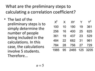
Downloaded 54 times


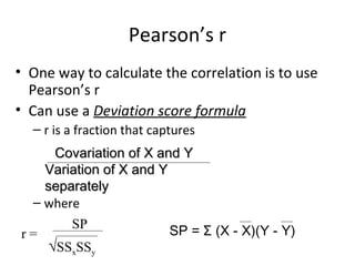
![The Computational Formula
( )( )
( )[ ] ( )[ ]∑ ∑∑ ∑
∑∑ ∑
−−
−
=
2222
YYnXXn
YXXYn
r](https://image.slidesharecdn.com/chapter12-140422114000-phpapp01/85/Chapter-12-20-320.jpg)
![( )( )
( )[ ] ( )[ ]∑ ∑∑ ∑
∑∑ ∑
−−
−
=
2222
YYnXXn
YXXYn
r
∑
∑
∑
∑
∑
=
=
=
=
=
=
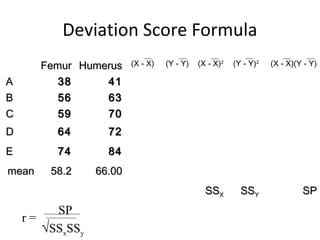
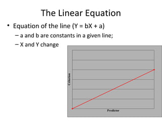
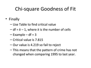
2465
3205
1985
125
95
5
2
2
XY
Y
X
Y
X
n
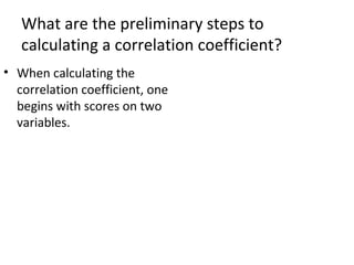
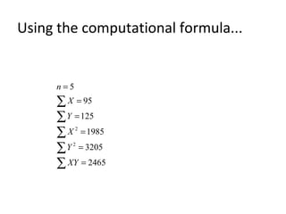
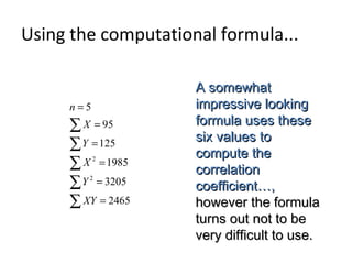
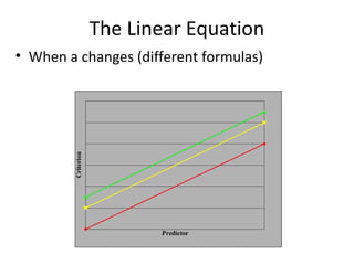
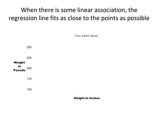
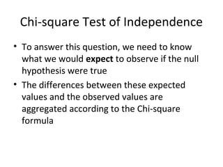
The formula is...The formula is...
Using the computational formula...](https://image.slidesharecdn.com/chapter12-140422114000-phpapp01/85/Chapter-12-37-320.jpg)
![( )( )
( )[ ] ( )[ ]∑ ∑∑ ∑
∑∑ ∑
−−
−
=
2222
YYnXXn
YXXYn
r
∑
∑
∑
∑
∑
=
=
=
=
=
=
2465
3205
1985
125
95
5
2
2
XY
Y
X
Y
X
n
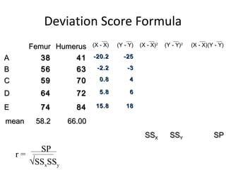
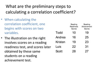
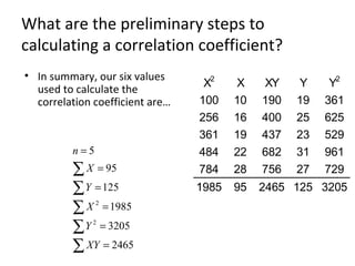
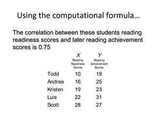
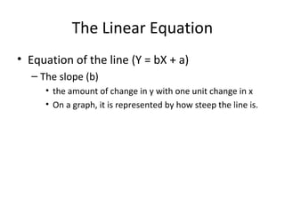
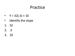
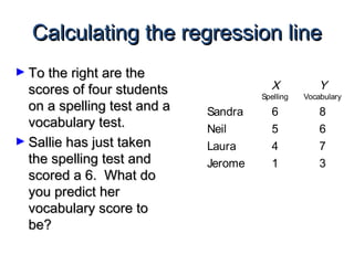
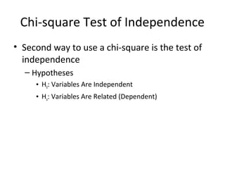
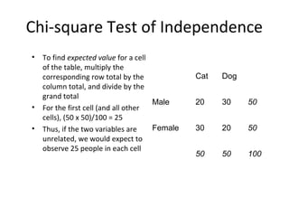
The variables in thisThe variables in this
formula consist of onlyformula consist of only
the six previouslythe six previously
calculated values to thecalculated values to the
left...left...
Using the computational formula...](https://image.slidesharecdn.com/chapter12-140422114000-phpapp01/85/Chapter-12-38-320.jpg)
![∑
∑
∑
∑
∑
=
=
=
=
=
=
2465
3205
1985
125
95
5
2
2
XY
Y
X
Y
X
n
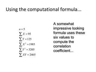
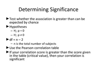
Here is the formula withHere is the formula with
these values inserted...these values inserted...
Using the computational formula...
( )( )
( )[ ] ( )[ ]∑ ∑∑ ∑
∑∑ ∑
−−
−
=
2222
YYnXXn
YXXYn
r
( )( ) ( )( )
( )( ) ( )[ ]( )( ) ( )[ ]22
125320559519855
1259524655
−−
−
=r](https://image.slidesharecdn.com/chapter12-140422114000-phpapp01/85/Chapter-12-39-320.jpg)

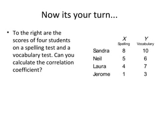
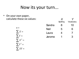
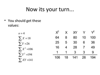
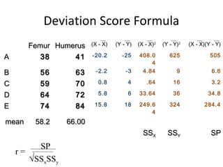
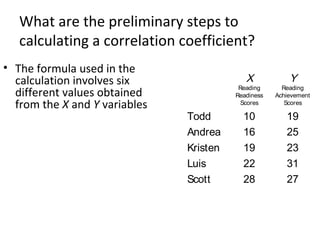
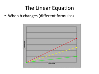
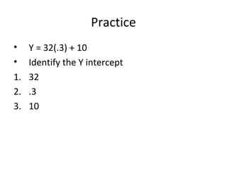
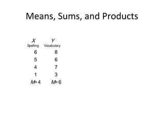
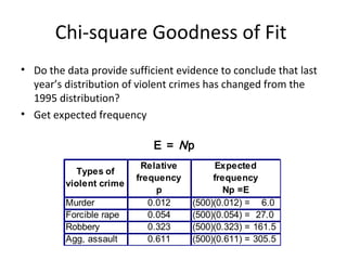
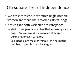
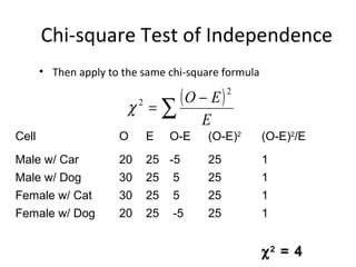
![Now its your turn...
• Now insert these values
in the equation
141
194
106
26
18
4
2
2
∑
∑
∑
∑
∑
=
=
=
=
=
=
XY
Y
X
Y
X
n
( )( )
( )[ ] ( )[ ]∑ ∑∑ ∑
∑∑ ∑
−−
−
=
2222
YYnXXn
YXXYn
r
( )( ) ( )( )
( )( ) ( )[ ]( )( ) ( )[ ]22
261944181064
26181414
−−
−
=r
96.0
100
96
==r](https://image.slidesharecdn.com/chapter12-140422114000-phpapp01/85/Chapter-12-46-320.jpg)

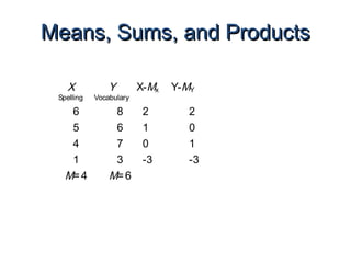
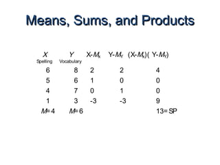
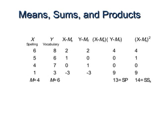
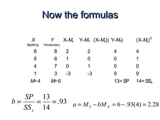


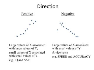
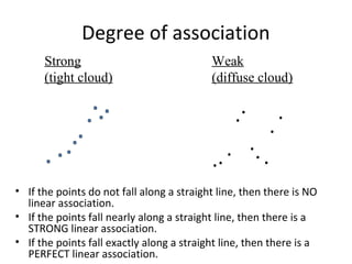
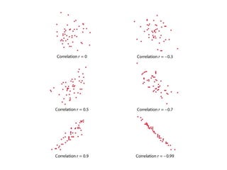
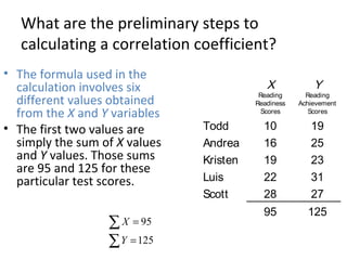
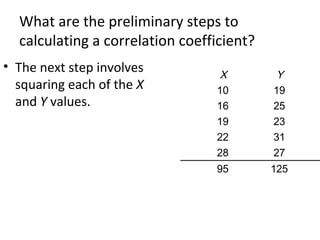
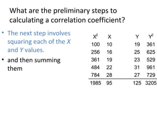
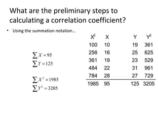
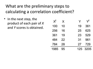
This document provides an overview of correlation, including: - Correlation measures the degree of linear relationship between two variables from -1 to 1. - It can be positive, negative, or zero. A stronger correlation is closer to -1 or 1. - Calculating correlation involves determining sums, means, and deviations of the variables to plug into the correlation formula. - The example calculates a correlation coefficient of 0.75 between reading readiness and achievement scores, indicating a strong positive linear relationship.