Downloaded 115 times
![6.1 LAPLACE’S AND POISSON’S EQUATIONS
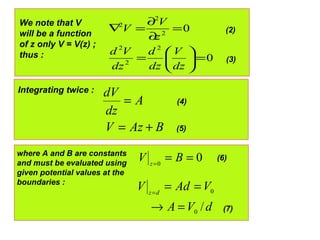
To derive Laplace’s and Poisson’s equations , we start with Gauss’s
law in point form :
vED ρε =•∇=•∇
VE −∇=Use gradient concept :
( )[ ]
ε
ρ
ρε
v
v
V
V
−=∇•∇
=∇−•∇
2
∇=∇•∇Operator :
Hence :
(1)
(2)
(3)
(4)
(5) => Poisson’s equation
is called Poisson’s equation applies to a homogeneous media.
22
/ mVV v
ε
ρ
−=∇](https://image.slidesharecdn.com/chap6laplaces-and-poissons-equations-130506065118-phpapp01/85/Chap6-laplaces-and-poissons-equations-3-320.jpg)
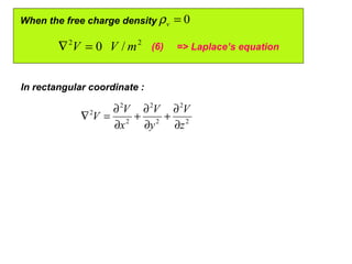
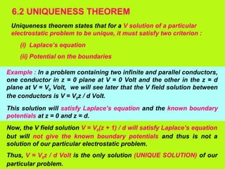
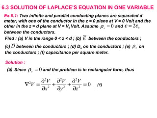
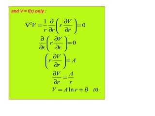
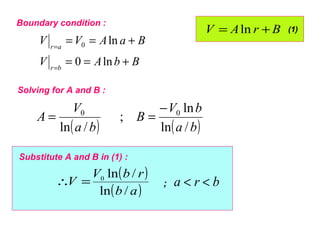
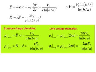
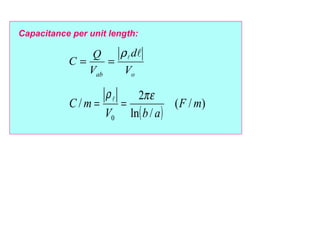
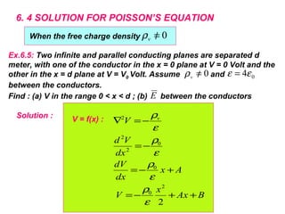
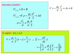
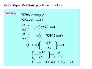
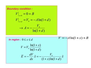

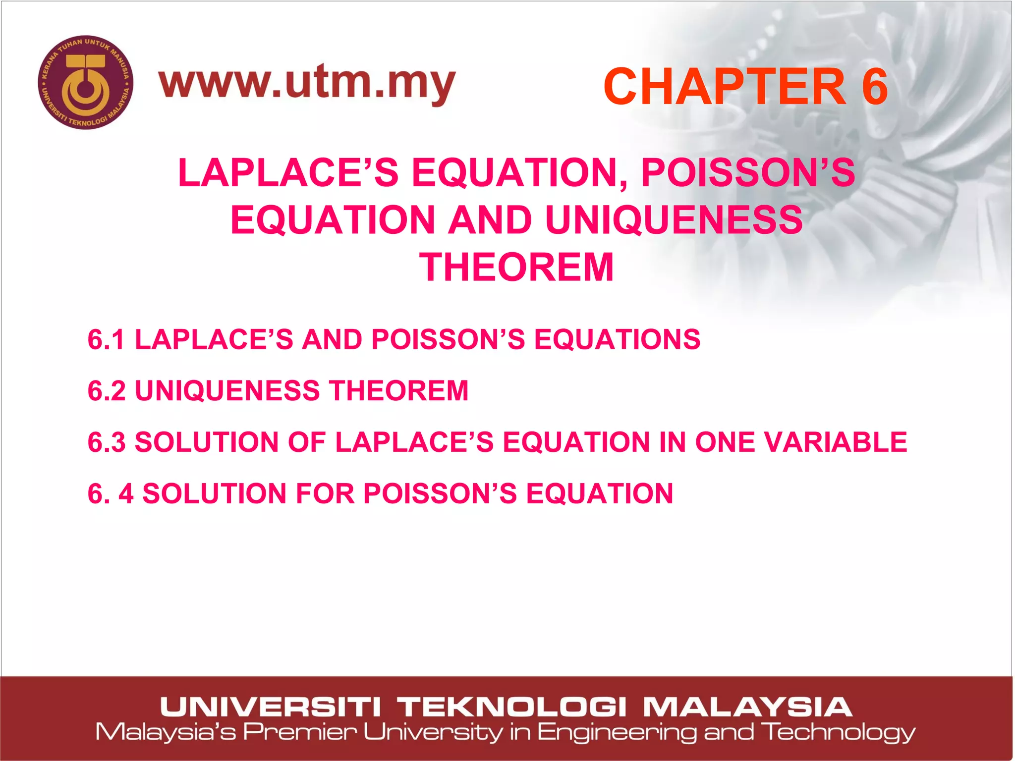
This document discusses Laplace's equation, Poisson's equation, and the uniqueness theorem. It begins by introducing Laplace's equation and Poisson's equation, which are derived from Gauss's law. Poisson's equation applies to problems with a non-zero charge density, while Laplace's equation applies when the charge density is zero. The uniqueness theorem states that for the potential solution to be unique, it must satisfy Laplace's equation and the known boundary conditions. Several examples are then provided to demonstrate solving Laplace's and Poisson's equations for different boundary value problems.