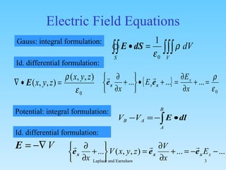
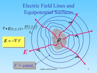
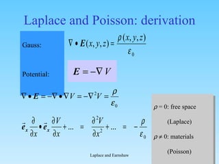
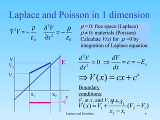
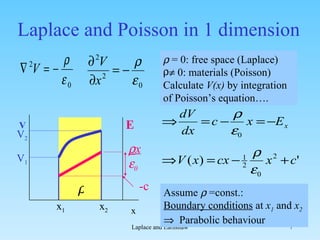
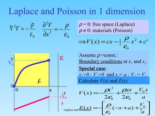
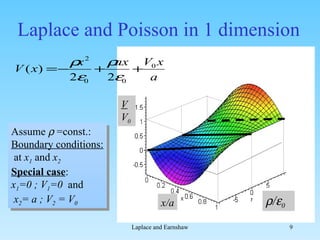
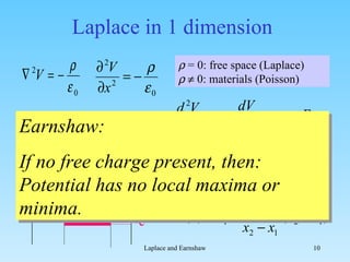
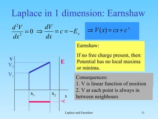
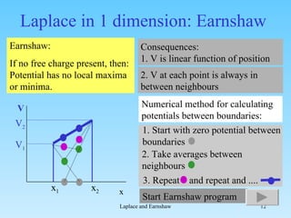
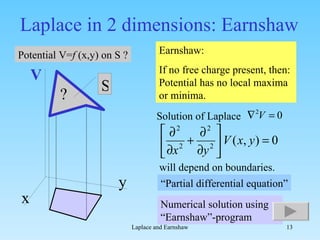
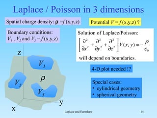
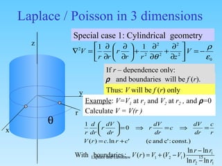
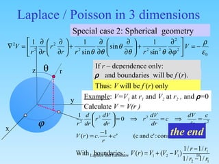
1. The document discusses Laplace's equation and Earnshaw's theorem regarding electric field and potential distributions. 2. Earnshaw's theorem states that without free charges, the electric potential cannot have local maxima or minima. 3. Numerical methods like the finite element method and Earnshaw program can be used to calculate electric potential distributions based on boundary conditions in one, two, and three dimensions.

1. Laplace Potential Distribution and Earnshaw’s Theorem © Frits F.M. de Mul

2. Laplace and Earnshaw Electric Field equations: Gauss’ Law and Potential Gradient Law Laplace and Poisson: derivation Laplace and Poisson in 1 dimension Charge-free space: Earnshaw’s Theorem Finite-Elements method for Potential Distribution Laplace and Poisson in 2 and 3 dimensions

3. Electric Field Equations Gauss: integral formulation: Potential: integral formulation: Id. differential formulation: Id. differential formulation:

4. Electric Field Lines and Equipotential Surfaces E  V = const .

5. Laplace and Poisson: derivation Gauss: Potential:  = 0: free space (Laplace)    0: materials (Poisson)

6. Laplace and Poisson in 1 dimension  = 0: free space (Laplace)   0: materials (Poisson) Calculate V(x) for  = 0 by integration of Laplace equation Boundary conditions : V 1 at x 1 and V 2 at x 2 : x 1 x 2 V 1 V 2 x V -c E

7. Laplace and Poisson in 1 dimension  = 0: free space (Laplace)  0: materials (Poisson) Calculate V(x) by integration of Poisson’s equation…. Assume  =const.: Boundary conditions at x 1 and x 2  Parabolic behaviour  x V x 1 x 2 V 1 V 2 E -c  x  0

8. Laplace and Poisson in 1 dimension  = 0: free space (Laplace)   0: materials (Poisson) Assume  =const.: Boundary conditions at x 1 and x 2 Special case : x 1 =0 ; V 1 =0 and x 2 = a ; V 2 = V 0 Calculate V(x) and E(x) x V 0 a 0 V 0  E -V 0 a

9. Laplace and Poisson in 1 dimension Assume  =const.: Boundary conditions: at x 1 and x 2 Special case : x 1 =0 ; V 1 =0 and x 2 = a ; V 2 = V 0  /  0 x/a V V 0

10. Laplace in 1 dimension  = 0: free space (Laplace)   0: materials (Poisson) Boundary conditions at x 1 and x 2 : Earnshaw: If no free charge present, then: Potential has no local maxima or minima. -c V 1 V 2 x V x 1 x 2 E

11. Laplace in 1 dimension: Earnshaw Earnshaw: If no free charge present, then: Potential has no local maxima or minima. Consequences: 1. V is linear function of position 2. V at each point is always in between neighbours x V x 1 x 2 V 1 V 2 -c E

12. Laplace in 1 dimension: Earnshaw Earnshaw: If no free charge present, then: Potential has no local maxima or minima. Consequences: 1. V is linear function of position 2. V at each point is always in between neighbours Numerical method for calculating potentials between boundaries: Start Earnshaw program x V x 1 x 2 V 1 V 2 1. Start with zero potential between boundaries 2. Take averages between neighbours 3. Repeat and repeat and ....

13. Laplace in 2 dimensions: Earnshaw Earnshaw: If no free charge present, then: Potential has no local maxima or minima. Potential V= f (x,y) on S ? Solution of Laplace will depend on boundaries. “ Partial differential equation” Numerical solution using “Earnshaw”-program V x y ? S

14. Laplace / Poisson in 3 dimensions Potential V = f (x,y,z) ? Boundary conditions: V 1 , V 2 and V 3 = f (x,y,z) Spatial charge density:  = f (x,y,z) Special cases: cylindrical geometry spherical geometry 4-D plot needed !? Solution of Laplace/Poisson: will depend on boundaries. z x y V 1 V 2 V 3 

15. Laplace / Poisson in 3 dimensions Special case 1: Cylindrical geometry If r – dependence only:  and boundaries will be f ( r ). Thus: V will be f ( r ) only Example : V=V 1 at r 1 and V 2 at r 2 , and  =0 Calculate V = V(r ) z r x y 

16. Laplace / Poisson in 3 dimensions Special case 2: Spherical geometry If r – dependence only:  and boundaries will be f ( r ). Thus: V will be f ( r ) only Example : V=V 1 at r 1 and V 2 at r 2 , and  =0 Calculate V = V(r ) the end z r x y  