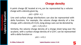
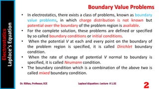
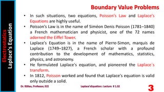
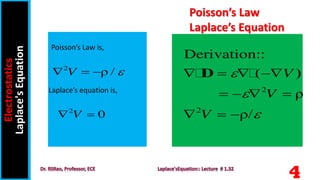
This document summarizes key concepts in electrostatics including Laplace's equation, Poisson's equation, and boundary value problems. It discusses: 1) Boundary value problems where the potential over a boundary is known but not the charge distribution, requiring boundary conditions to solve. 2) Laplace's equation and Poisson's equation, important for solving boundary value problems. Laplace's equation describes the electric potential in static systems with no charges while Poisson's equation includes the charge density. 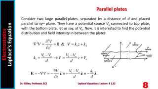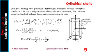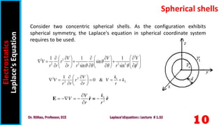3) Methods for solving problems involving different charge distributions and geometries like parallel plates, cylindrical shells, and spherical shells using Laplace's equation and appropriate coordinate systems.

1. Series: EMF Theory
Lecture: #1.32
Dr R S Rao
Professor, ECE
ELECTROSTATICS
Passionate
Teaching
Joyful
Learning
Laplace’s equation, Poisson’s equation, direct integration method,
application to parallel plates, cylindrical shells, spherical shells.

2. 2
• In electrostatics, there exists a class of problems, known as boundary
value problems, in which charge distribution is not known but
potential over the boundary of the problem region is available.
• For the complete solution, these problems are defined or specified
by so called boundary conditions or initial conditions.
• When the potential V at each and every point on the boundary of
the problem region is specified, it is called Dirichlet boundary
condition.
• When the rate of change of potential V normal to boundary is
specified, it is called Neumann condition.
• The boundary condition which is a combination of the above two is
called mixed boundary condition.
Electrostatics
Laplace's
Equation Boundary Value Problems

3. 3
• In such situations, two equations, Poisson's Law and Laplace's
Equations are highly useful.
• Poisson's Law is in the name of Siméon Denis Poisson (1781–1840)
a French mathematician and physicist, one of the 72 names
adorned the Eiffel Tower.
• Laplace's Equation is in the name of Pierre-Simon, marquis de
Laplace (1749–1827), a French scholar with a profound
contribution to the development of mathematics, statistics,
physics, and astronomy.
• He formulated Laplace's equation, and pioneered the Laplace´s
transform.
• In 1812, Poisson worked and found that Laplace's equation is valid
only outside a solid.
Electrostatics
Laplace's
Equation Boundary Value Problems

4. 2
ρ /
V 
  
Electrostatics
Laplace's
Equation
2
0
V
 
Laplace’s equation is,
Poisson’s Law is,
2
2
Derivation::
(
ρ
ρ/
V
V
V



   
   
  
D )
Poisson’s Law
Laplace’s Equation
4

5. 5
Similarly, the volume charge density of a charge sheet lying over the
xy-plane, with a surface charge density of σ C/m2, can be represented
with a delta function as
ρ( ) ( )
o
Q
 
r r r
ρ( ) λ ( ) ( )
y z
 

r
ρ( ) σ ( )
z


r
A point charge QC located at r=ro can be represented by a volume
charge with a density given by,
Line and surface charge distributions can also be represented with
delta functions. For example, the volume charge density of a line
charge, with a density of λ C/m, lying along x-axis can be denoted by
Electrostatics
Laplace's
Equation Charge density

6. • This theorem has special importance in boundary value problems in assuring
the uniqueness of their solutions.
• It states that ′within some closed region, a solution to Laplace equation or
Poisson equation for the potential function V is the only solution that
satisfies the potential specified over the boundaries of the region′.
• Thus, it assures the uniqueness of the solution obtained by solving Laplace's
Law or Poisson´s equation for a given boundary conditions.
Electrostatics
Laplace's
Equation Uniqueness Theorem
6

7. • Direct integration method falls in the category of boundary value problems.
• This method is limited to one-dimensional problems.
• In this method Laplace´s equation is used to find field intensity.
• Here, a few configurations of conductors are examined to illustrate the utility
of this method in estimating the potential distribution and consequently
field intensity.
Electrostatics
Laplace's
Equation Direct integration
7

8. 2
2
1 2
2
0 &
V
V V k z k
z

    

1 1
1
o o
o
V V V V
k V z V
d d
 
   
1 1
ˆ ˆ ˆ
o
V V k
V
V
z d d


     

E z = z = z
Electrostatics
Laplace's
Equation Parallel plates
Consider two large parallel-plates, separated by a distance of d and placed
parallel to xy– plane. They have a potential source V1 connected to top plate,
with the bottom plate, let us say, at Vo. Now, it is interested to find the potential
distribution and field intensity in between the plates.
8

9. 2 2
2
2 2 2
1 1
V V V
V
z

    
 
 
   
   
 
 
   
   
2
1 2
1
0 & ln
V
V V k k
 
  
 
 
    
 
 
 
1
ˆ ˆ
k
V
V
 

    

E ρ = ρ
Cylindrical shells
Electrostatics
Laplace's
Equation
Consider finding the potential distribution between coaxial cylindrical
conductors. As the configuration exhibits cylindrical symmetry, the Laplace′s
equation in cylindrical coordinate system requires to be used.
9

10. 2
2 2
2 2 2 2 2
1 1 1
sin
sin sin
V V V
V r
r r r r r

    
 
    
   
     
   
    
     
2 2 1
2
2
1
0 &
k
V
V r V k
r r r r
 
 
    
 
 
 
1
2
ˆ ˆ
k
V
V
r r

    

E r = r
Spherical shells
Electrostatics
Laplace's
Equation
Consider two concentric spherical shells. As the configuration exhibits
spherical symmetry, the Laplace's equation in spherical coordinate system
requires to be used.
10

11. ENOUGH
FOR
TODAY
ENOUGH
FOR
TODAY
ENOUGH
FOR
TODAY
ENOUGH
FOR
TODAY
ENOUGH
FOR
TODAY
11