Downloaded 197 times


![Example
Imagine an electromagnetic plane wave in vacuum whose electric field (in
SI units) is given by
0,0),109103(sin10 1462
zyx EEtzE
Determine (i) the speed, frequency, wavelength, period, initial phase and
electric field amplitude and polarization, (ii) the magnetic field.
Solution
(i) The wave function has the form: )(sin),( 0 vtzkEtzE xx
)]103(103sin[10Here, 862
tzEx
1816
ms103,m103
vk
Hz105.4,nm7.666
2 14
v
f
k](https://image.slidesharecdn.com/electromagneticwaves-160913110902/85/Electromagnetic-waves-16-320.jpg)


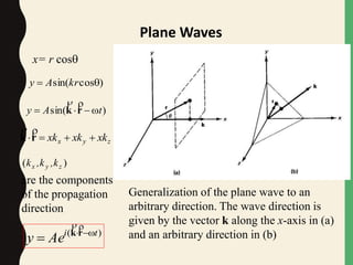
sin( tkxAy
A = amplitude k = 2/ (propagation constant)
)](cos[ txkAy vor
v = f = f (2/k) k v = 2f = (angular frequency)
)cos( tkxAy or
Phase : = k(x + vt) = kx + t moving in the – x-direction
= k(x - vt) = kx - t moving in the + x-direction](https://image.slidesharecdn.com/electromagneticwaves-160913110902/85/Electromagnetic-waves-25-320.jpg)


![yxE ˆˆ
~ )(
0
)(
0
yx
tkzi
y
tkzi
x eEeE
)(
0
)(
00
~~
ˆˆ[
~
tkzi
tkzii
y
i
x
e
eeEeE yx
EE
]yxE
]ˆˆ[
~
000 yxE yx
i
y
i
x eEeE
= complex amplitude vector for the polarized wave
Since the state of polarization of the light is completely determined
by the relative amplitudes and phases of these components, we
just concentrate only on the complex amplitude, written as a two-
element matrix – called Jones vector:
y
x
i
y
i
x
y
x
eE
eE
E
E
0
0
0
0
0 ~
~
~
E
Mathematical Representation of Polarized Light](https://image.slidesharecdn.com/electromagneticwaves-160913110902/85/Electromagnetic-waves-32-320.jpg)


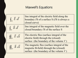
Maxwell derived a set of equations that unified electricity, magnetism and light as manifestations of electromagnetic waves. His equations predicted that changes in electric and magnetic fields propagate as waves at the speed of light. This supported Maxwell's theory that light itself is an electromagnetic wave. The electromagnetic spectrum encompasses all possible frequencies of electromagnetic waves, from radio waves to gamma rays. Maxwell's equations form the basis for the modern understanding of electromagnetism and optics.


