Downloaded 238 times


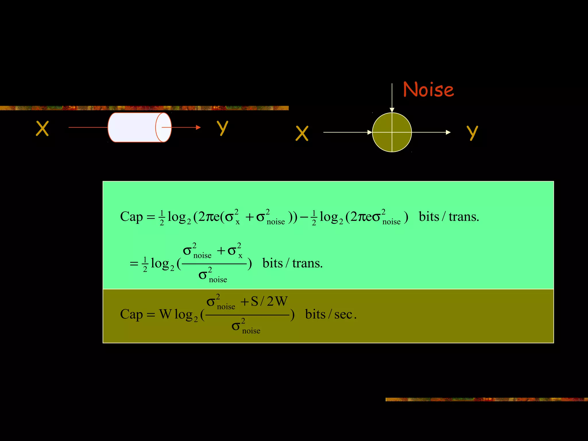
![Capacity for Additive White Gaussian Noise
Noise
Input X Output Y
Cap := sup [H(Y) − H( Noise)]
p( x )
x 2 ≤S / 2 W W is (single sided) bandwidth
Input X is Gaussian with power spectral density (psd) ≤S/2W;
Noise is Gaussian with psd = σ2noise
Output Y is Gaussian with psd = σy2 = S/2W + σ2noise
For Gaussian Channels: σy2 = σx2 +σnoise2](https://image.slidesharecdn.com/channel-coding-130214001651-phpapp01/75/Channel-coding-29-2048.jpg)

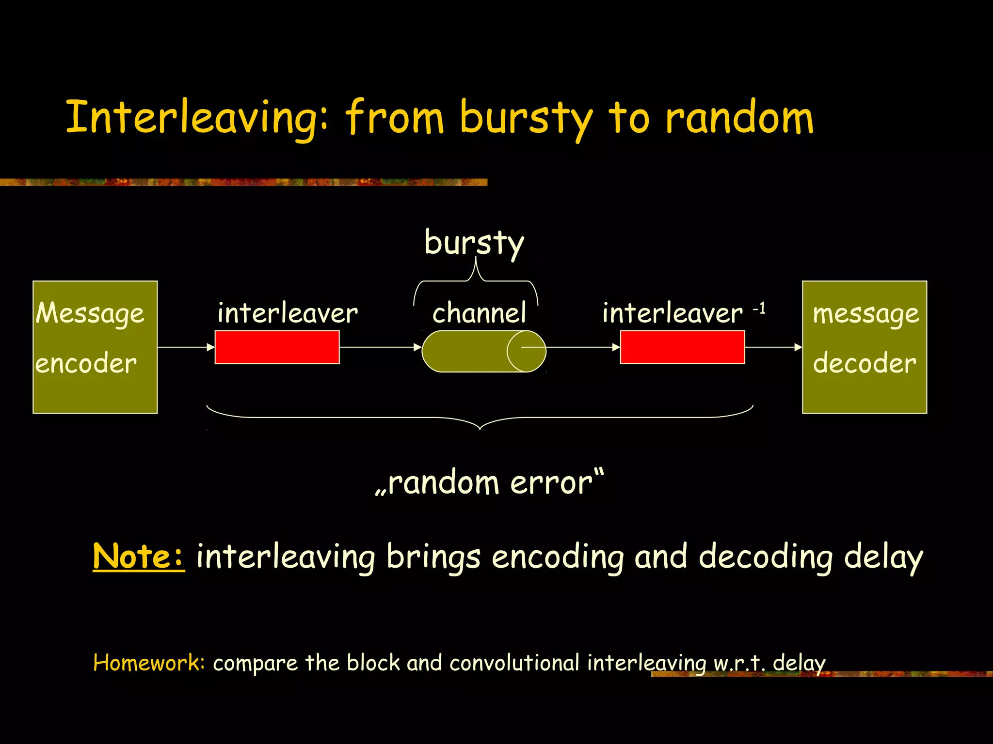
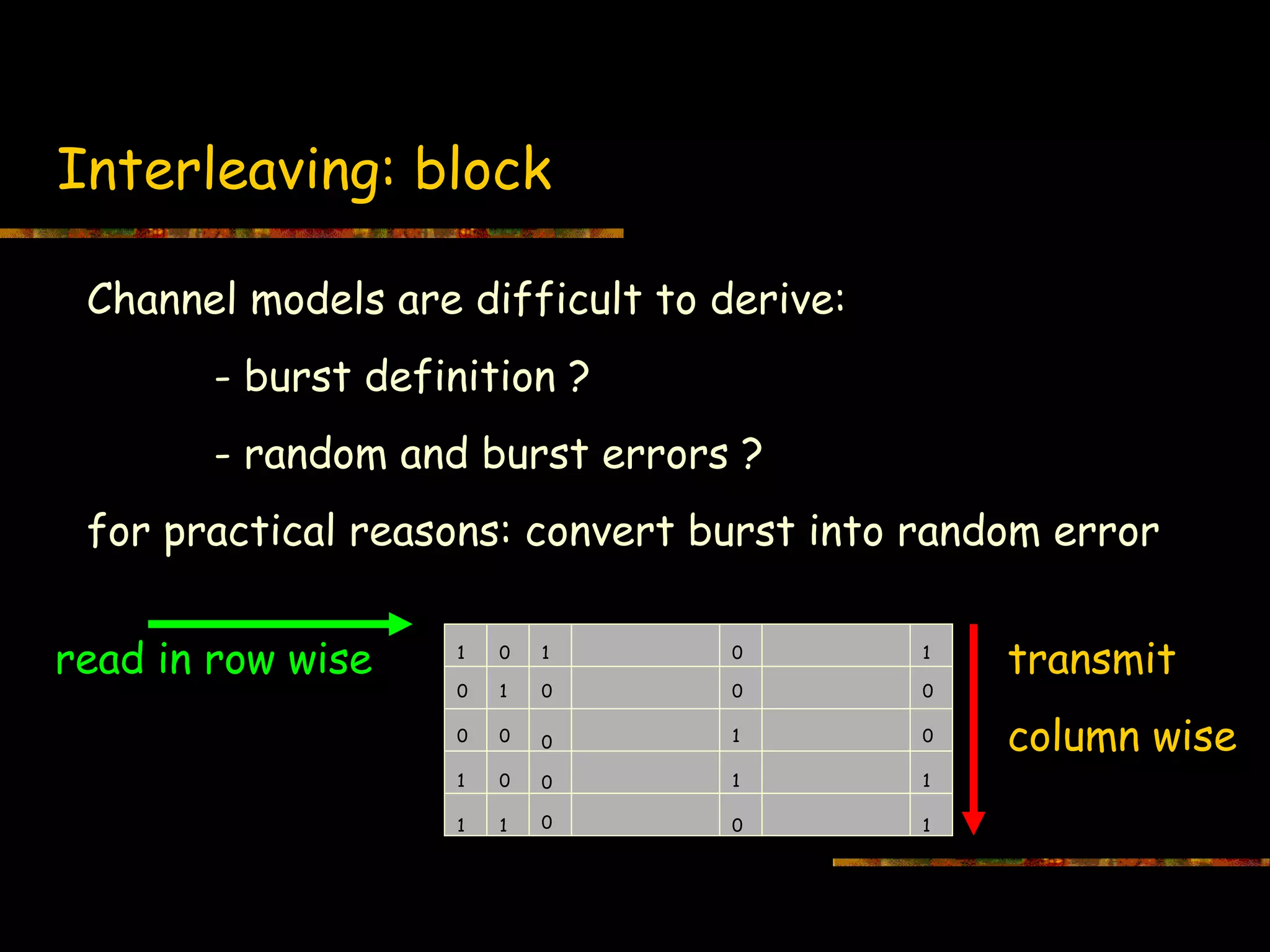
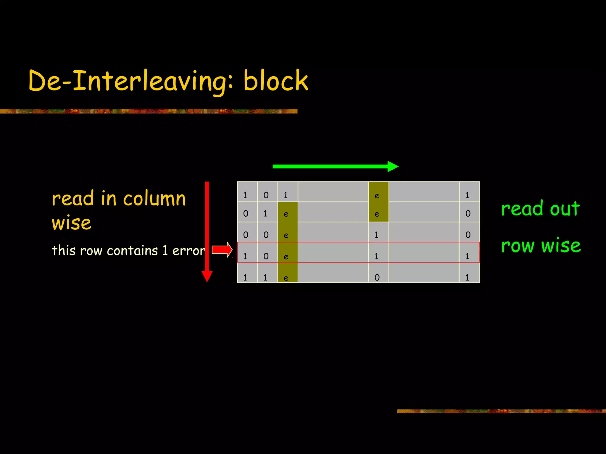
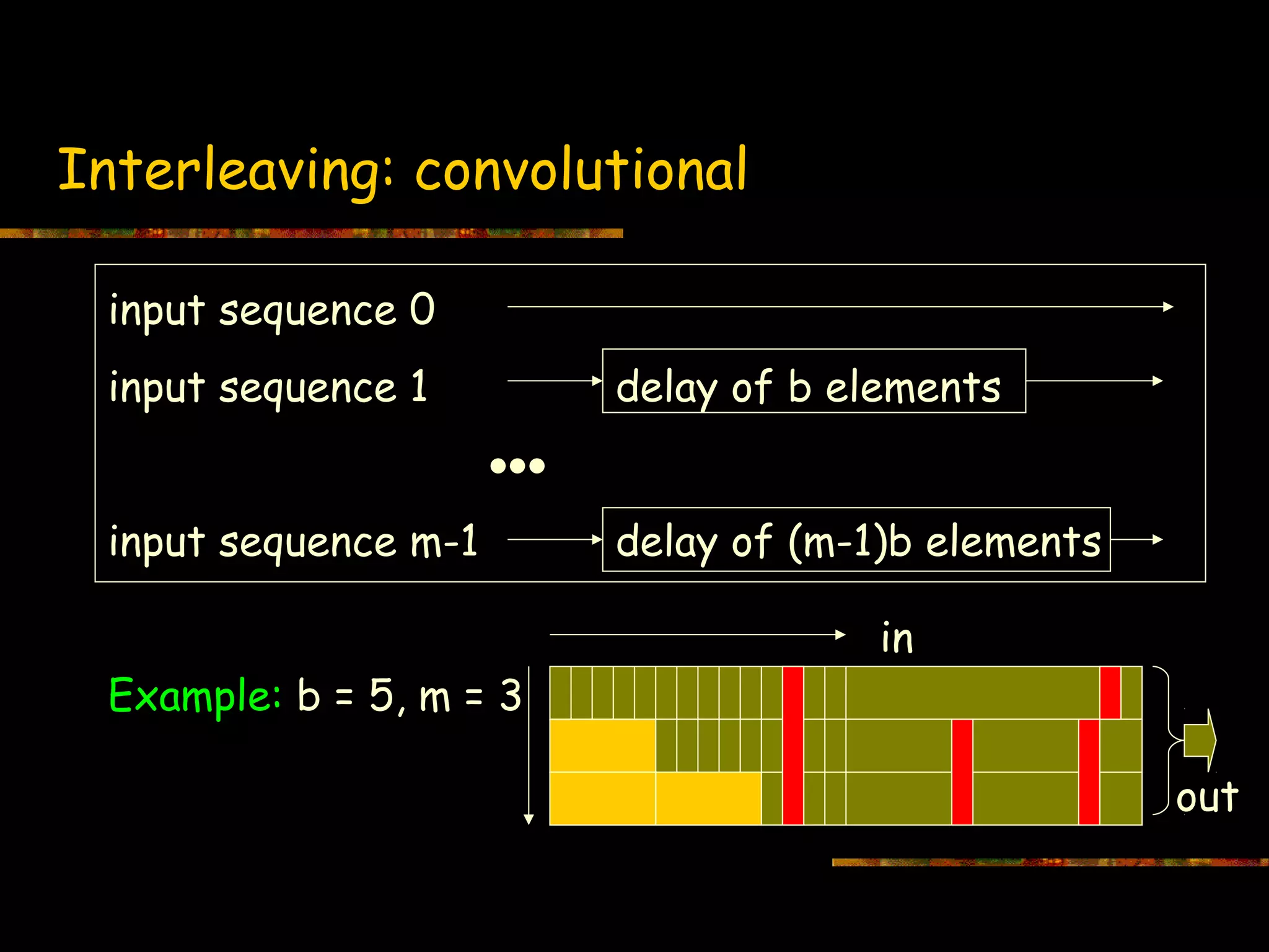

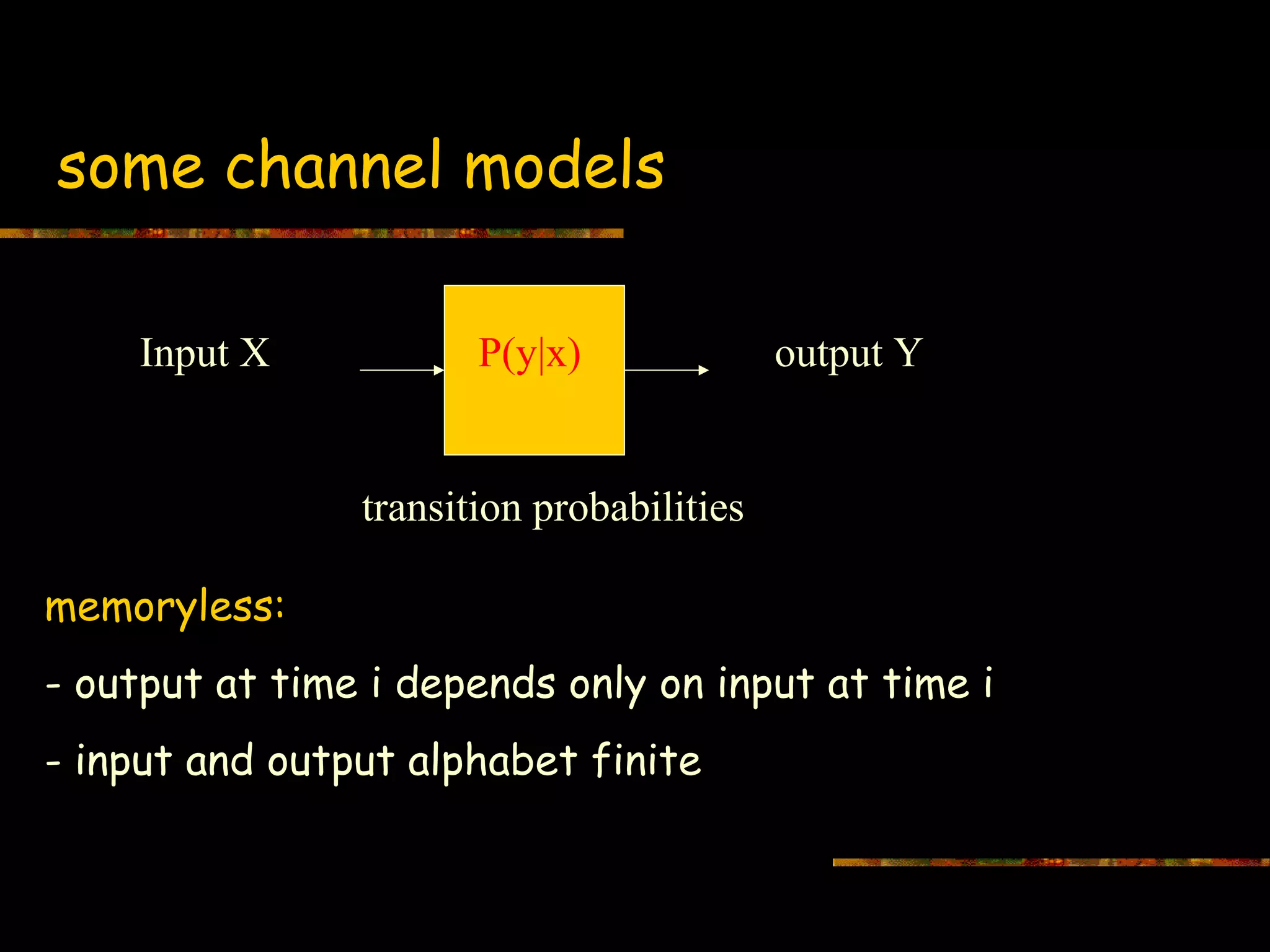
This document introduces information theory and channel capacity models. It discusses several channel models including the binary symmetric channel (BSC), binary erasure channel, and additive white Gaussian noise channel. It explains how channel capacity is defined as the maximum rate of error-free transmission and derives the capacity for some basic channels. The document also covers channel coding techniques like interleaving that can improve performance by converting burst errors into random errors.