Downloaded 51 times

![these rather than by the noise. Thus, we say that a mature cellular system is
interference limited rather than noise limited. Keeping this interference
below a certain level is done partly by controlling the channel re–use
distance. The larger D is, the less is the interference.
Reflected channel interference or C/R is the relation between the signal
strength of the desired signal C and the reflected signal R. This
phenomenon is referred to as time dispersion. Actually, there is no
difference in interference caused by co-channel interference or by reflected
channel interference. The result is the same: energy disturbing our desired
signal in the very same frequency domain. This disturbances might effect
the possible re-use distance in the same way as C/I
5.6 Capacity calculation for cellular network
One starting point when designing a cellular network is the estimation of
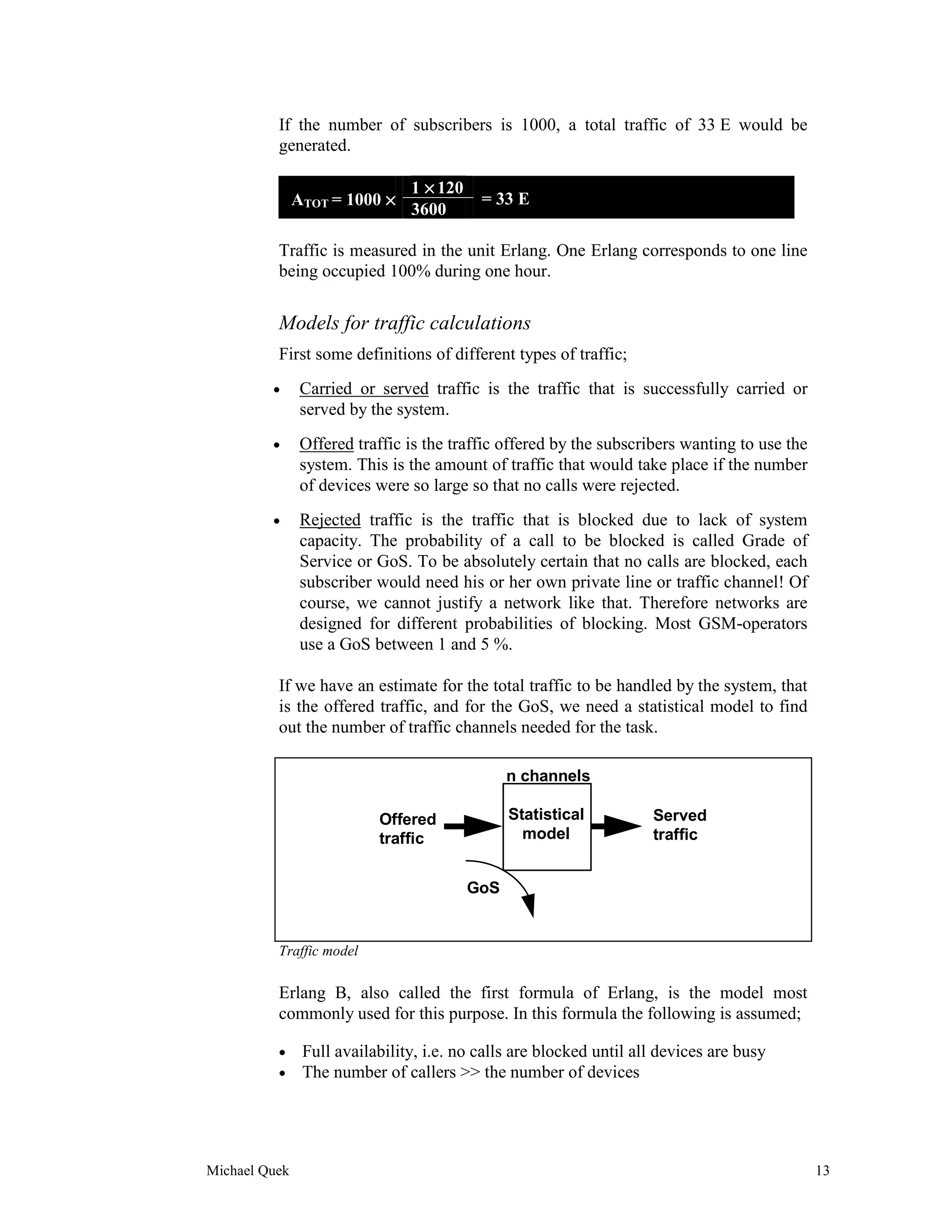
traffic. To be able to offer a certain traffic capacity with a certain quality,
some kind of statistical model to figure out the number of required
channels is needed. When dealing with GSM we need to handle not only
traffic capacity, but also the capacity of the control channels needed to set
up the call. Traffic theory gives us a chance to calculate on traffic, and
from the results base our dimensioning of the network. The calculations
should be based on the busy hour of the network.
Definition of traffic
When estimating the traffic offered by one subscriber, the call intensity γ
and the average duration τ of each call are essential. One way of defining
traffic is this:
γ ×τ
ASUB = [E]
3600
ASUB = traffic from one subscriber
γ = number of calls per hour per subscriber
τ = average call duration
Typical values could be:
γ: 1
τ: 120 seconds
×
1× 120
ASUB = = 33 mE
3600
Michael Quek 12](https://image.slidesharecdn.com/5-cellplanning-130327230743-phpapp02/75/Cell-Planning-12-2048.jpg)

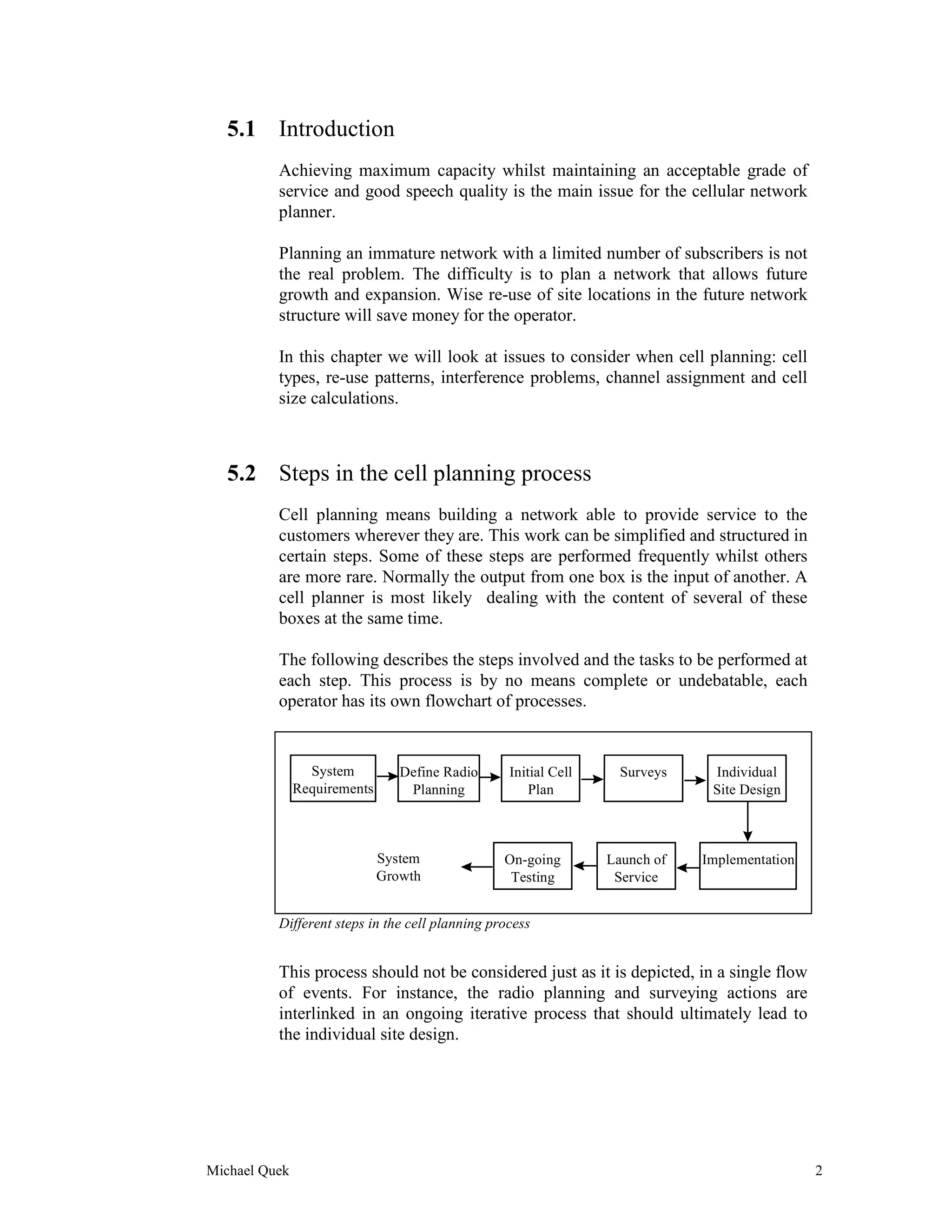
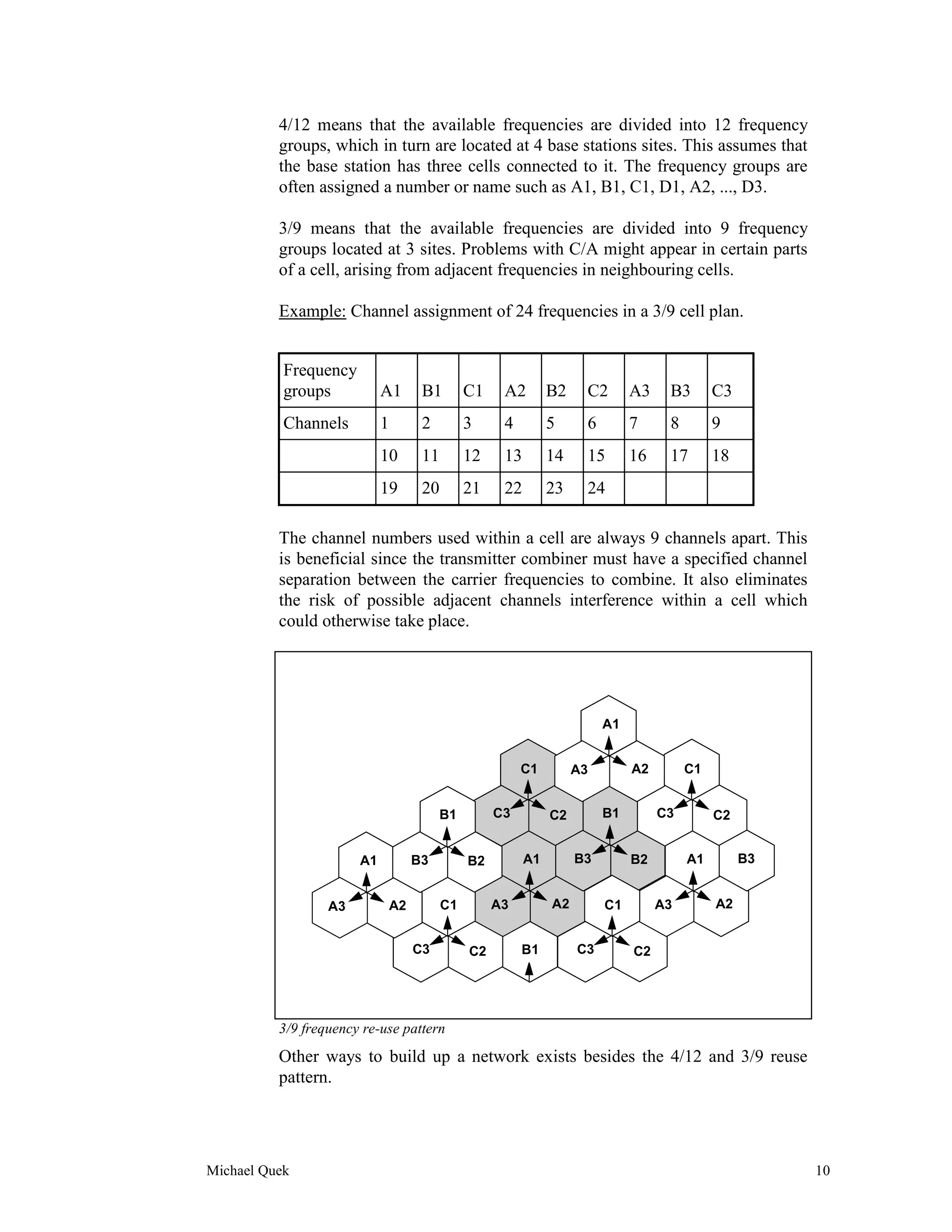
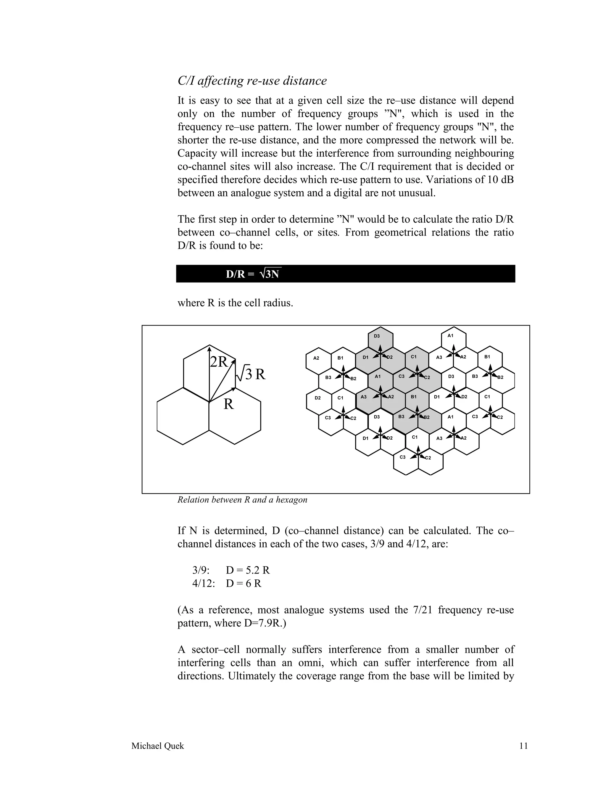
The document discusses cell planning in cellular networks. It covers key steps in the cell planning process including defining system requirements, radio planning guidelines, performing initial cell planning and surveys, and designing individual sites. It also discusses factors that influence cell planning such as different cell types (macro, micro, pico), interference between cells, frequency reuse patterns, and calculating coverage and capacity. The optimal cell plan balances coverage, capacity, cost, and quality of service according to the operator's needs.


