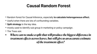
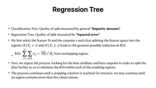
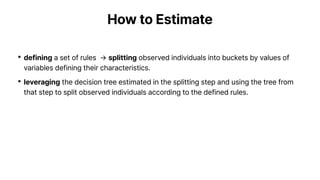
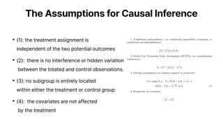
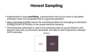
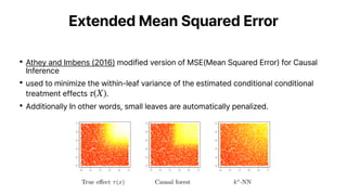
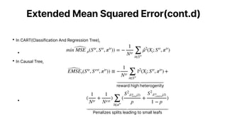
Bongho Lee
Introduction to Causal
Random Forest
Causal Inference Study
Causal Random Forest
•Random forest for Causal Inference, especially to calculate heterogeneous effect.
•Useful when there are lots of confounding variables.
•Split strategy is the key idea.
•mostly used to identify sub group in marketing or policy campaign.
•The Trees ask:
• Wherecanwemakeasplitthatwillproducethebiggestdi
ff
erencein
treatmente
ff
ectsacrossleaves,butstillgiveusanaccurateestimate
ofthetreatmente
ff
ect?
Heterogeneous Treatment Effect
•Many studies estimate an average treatment effect (ATE).
•The treatment effect within subgroups may vary considerably from the ATE.
•The study of treatment effect heterogeneity is the study of these differences across
subjects: For whom are there big effects?
OLS( Ordinary Least Squares)
•Simplest Way to Calculate ATE(Average Treatment Effect)
•How to estimate whether discount affects spend
•In python, smf.ols(‘spend ~ discount', df).fit().summary()
time device browser region discount spend
10.78mobile edge 9 0 0.46
0.57desktop firefox 9 1 11.04
3.74mobile safari 7 0 1.81
13.37desktop other 5 0 31.90
0.71mobile explorer 2 0 15.42
The Limitation of OLS
•How to estimate whether discount by device affects spend?
•smf.ols('spend ~ discount * device', df).fit().summary()
• Splitting is easy for categorical variables, but for a continuous variable
like ‘time’?
•it is not intuitive where to split. Every hour? And which dimension is more informative?
• Data Speaks!
→
The motivation to use causal random forest
Regression Tree
• Classi
fi
cation Tree: Quality of split measured by general “Impurity measure"
• Regression Tree: Quality of split measured by “Squared error”
• We
fi
rst select the feature Xi and the cutpoint s such that splitting the feature space into the
regions { } and { } leads to the greatest possible reduction in RSS.
• RSS: , : Non overlapping region,
• Next, we repeat the process, looking for the best attribute and best cutpoint in order to split the
data further so as to minimize the RSS within each of the resulting regions.
• The process continues until a stopping criterion is reached; for instance, we may continue until
no region contains more than
fi
ve observations.
X|Xi < s X|Xi ≥ s
J
∑
i=1
∑
j∈Ri
(yj − ̂
YRi )2
Rj
How to Estimate
•defining a set of rules → splitting observed individuals into buckets by values of
variables defining their characteristics.
•leveraging the decision tree estimated in the splitting step and using the tree from
that step to split observed individuals according to the defined rules.
The Assumptions for Causal Inference
•(1): the treatment assignment is
independent of the two potential outcomes
•(2): there is no interference or hidden variation
between the treated and control observations.
•(3): no subgroup is entirely located
within either the treatment or control group
•(4): the covariates are not affected
by the treatment
The Difference from Traditional Tree
•Honest Sampling
•Extended Mean Squared Error
Honest Sampling
•Implemented to avoid overfitting, a phenomenon that occurs when a calculated
estimation does not extrapolate well to a general population.
•Athey and Imbens(2016) resolve the overfitting problem by leveraging an estimation
strategy known as honesty in the causal inference literature.
•The estimating subsample is used in the estimating step of causal inference with
decision trees and, as previously described, this data is used to generate unbiased
CATE estimates.
Extended Mean Squared Error
•Athey and Imbens (2016) modified version of MSE(Mean Squared Error) for Causal
Inference
•used to minimize the within-leaf variance of the estimated conditional conditional
treatment effects .
•Additionally In other words, small leaves are automatically penalized.
τ(X)
Extended Mean Squared Error(cont.d)
•In CART(Classification And Regression Tree),
•
•In Causal Tree,
•
min ̂
MSE μ(Ste
, Str
, πtr
)) = −
1
Ntr ∑
i∈Str
̂
μ2
(Xi; Str
, πtr
)
̂
EMSEτ(Ste
, Sest
, πtr
)) ≡ −
1
Ntr ∑
i∈Str
̂
τ2
(Xi; Str
, πtr
)
reward high heterogenity
+
(
1
Ntr
+
1
Nest
)
∑
l∈πtr
(
S2
𝒮
tr
treat(l)
p
+
S2
𝒮
tr
control(l)
1 − p
)
Penalizes splits leading to small leafs
Implementation
•Requirement: EconML (Warning: Not executable on Apple Silicon)
•Colab Link: Causal Tree
References
•A Leader's Guide to Heterogeneous Treatment Effects
•Causal Tree Learning For Heterogeneous Treatment Effect Estimation
•Athey and Imbens (2016)
•From Causal Trees to Forests

Causal Random Forest

  • 1.
    Bongho Lee Introduction toCausal Random Forest Causal Inference Study
  • 2.
    Causal Random Forest •Randomforest for Causal Inference, especially to calculate heterogeneous effect. •Useful when there are lots of confounding variables. •Split strategy is the key idea. •mostly used to identify sub group in marketing or policy campaign. •The Trees ask: • Wherecanwemakeasplitthatwillproducethebiggestdi ff erencein treatmente ff ectsacrossleaves,butstillgiveusanaccurateestimate ofthetreatmente ff ect?
  • 3.
    Heterogeneous Treatment Effect •Manystudies estimate an average treatment effect (ATE). •The treatment effect within subgroups may vary considerably from the ATE. •The study of treatment effect heterogeneity is the study of these differences across subjects: For whom are there big effects?
  • 4.
    OLS( Ordinary LeastSquares) •Simplest Way to Calculate ATE(Average Treatment Effect) •How to estimate whether discount affects spend •In python, smf.ols(‘spend ~ discount', df).fit().summary() time device browser region discount spend 10.78mobile edge 9 0 0.46 0.57desktop firefox 9 1 11.04 3.74mobile safari 7 0 1.81 13.37desktop other 5 0 31.90 0.71mobile explorer 2 0 15.42
  • 5.
    The Limitation ofOLS •How to estimate whether discount by device affects spend? •smf.ols('spend ~ discount * device', df).fit().summary() • Splitting is easy for categorical variables, but for a continuous variable like ‘time’? •it is not intuitive where to split. Every hour? And which dimension is more informative? • Data Speaks! → The motivation to use causal random forest
  • 6.
    Regression Tree • Classi fi cationTree: Quality of split measured by general “Impurity measure" • Regression Tree: Quality of split measured by “Squared error” • We fi rst select the feature Xi and the cutpoint s such that splitting the feature space into the regions { } and { } leads to the greatest possible reduction in RSS. • RSS: , : Non overlapping region, • Next, we repeat the process, looking for the best attribute and best cutpoint in order to split the data further so as to minimize the RSS within each of the resulting regions. • The process continues until a stopping criterion is reached; for instance, we may continue until no region contains more than fi ve observations. X|Xi < s X|Xi ≥ s J ∑ i=1 ∑ j∈Ri (yj − ̂ YRi )2 Rj
  • 7.
    How to Estimate •defininga set of rules → splitting observed individuals into buckets by values of variables defining their characteristics. •leveraging the decision tree estimated in the splitting step and using the tree from that step to split observed individuals according to the defined rules.
  • 8.
    The Assumptions forCausal Inference •(1): the treatment assignment is independent of the two potential outcomes •(2): there is no interference or hidden variation between the treated and control observations. •(3): no subgroup is entirely located within either the treatment or control group •(4): the covariates are not affected by the treatment
  • 9.
    The Difference fromTraditional Tree •Honest Sampling •Extended Mean Squared Error
  • 10.
    Honest Sampling •Implemented toavoid overfitting, a phenomenon that occurs when a calculated estimation does not extrapolate well to a general population. •Athey and Imbens(2016) resolve the overfitting problem by leveraging an estimation strategy known as honesty in the causal inference literature. •The estimating subsample is used in the estimating step of causal inference with decision trees and, as previously described, this data is used to generate unbiased CATE estimates.
  • 11.
    Extended Mean SquaredError •Athey and Imbens (2016) modified version of MSE(Mean Squared Error) for Causal Inference •used to minimize the within-leaf variance of the estimated conditional conditional treatment effects . •Additionally In other words, small leaves are automatically penalized. τ(X)
  • 12.
    Extended Mean SquaredError(cont.d) •In CART(Classification And Regression Tree), • •In Causal Tree, • min ̂ MSE μ(Ste , Str , πtr )) = − 1 Ntr ∑ i∈Str ̂ μ2 (Xi; Str , πtr ) ̂ EMSEτ(Ste , Sest , πtr )) ≡ − 1 Ntr ∑ i∈Str ̂ τ2 (Xi; Str , πtr ) reward high heterogenity + ( 1 Ntr + 1 Nest ) ∑ l∈πtr ( S2 𝒮 tr treat(l) p + S2 𝒮 tr control(l) 1 − p ) Penalizes splits leading to small leafs
  • 13.
    Implementation •Requirement: EconML (Warning:Not executable on Apple Silicon) •Colab Link: Causal Tree
  • 14.
    References •A Leader's Guideto Heterogeneous Treatment Effects •Causal Tree Learning For Heterogeneous Treatment Effect Estimation •Athey and Imbens (2016) •From Causal Trees to Forests