The document provides an overview of random forests, including the random forest recipe, why random forests work, and ramifications of random forests. The random forest recipe involves drawing bootstrap samples to grow trees, randomly selecting features at each split, and aggregating predictions. Random forests work by decorrelating trees, which reduces variance and leads to lower prediction error compared to individual trees. Ramifications discussed include using out-of-bag samples to estimate generalization error and calculating variable importance.

1. Random Forests
by Jaehyeong Ahn
Department of Applied Statistics, Konkuk University
jayahn0104@gmail.com
1 / 39

2. Random Forests
Topics to be covered
• Random forest recipe
• Why do random forests work?
• Ramifications of random forests
• Out-of-bag error estimate
• Variable importance
• Proximity
• Missing value imputation
• Outliers
• Unsupervised learning
• Balancing prediction error
2 / 39

3. Random Forest Recipe
Notations
• D = {(x(i)
, y(i)
)}N
i= be the data
• x(i)
∈ X and y(i)
∈ Y
• X is the input space with p features and Y is the output space
• Y = Rn
, in regression
• Y is a discrete finite set of K elements, in classification
• D(k): a bootstrapped sample, called the k-th ”in-bag” set
• OOB(k): the set of data points not in D(k), called the k-th
”out-of-bag” set
D = D(k) ∪ OOB(k), D(k) ∩ OOB(k) = ∅
• Regulate a parameter
• m p
• Fix some constants
• Nmin
• B
3 / 39

4. Random Forest Recipe
The way Random Forest works
Do for k =  to B
• Draw a bootstrap resample D(k) from D
• Grow a tree Tk using D(k) by applying the following splitting rule:
• At each node, randomly select m features (out of total p
features)
• Split the node by choosing the split that minimizes the
empirical risk among all possible splits using only these m
selected features
• Stop splitting the node if the terminal node contains fewer
than Nmin elements. Where Nmin is a predetermined number
• Do not prune
• From each tree Tk, get the predictor ϕk for k = , · · · , B
4 / 39

5. Get the final predictor ζ(x) :
• For regression:
ζ(x) = Avk{ϕk(x)} =

B
B
k=
ϕk(x)
• For classification:
ζ(x) = Plurk{ϕk(x)} = argmax
j∈Y
|{k : ϕk(x) = j}|
5 / 39

6. Why do random forests work?
Case A: Regression
• Preparation, Before get into the main idea
• Let us write ϕk(x) gotten out of D(k) as ϕ(x, θk)
• θk stands for all those things that were involved in the
construction of ϕk(x)
• Treating θ as a random variable, we write ϕ(x, θ)
• We don’t need to specify the distribution of θ as it is used only
a theoretical background
• But we can talk about the expectation Eθϕ(x, θ) of ϕ(x, θ)
with respect to θ and the probability Pθ(ϕ(X, θ) = j)
6 / 39

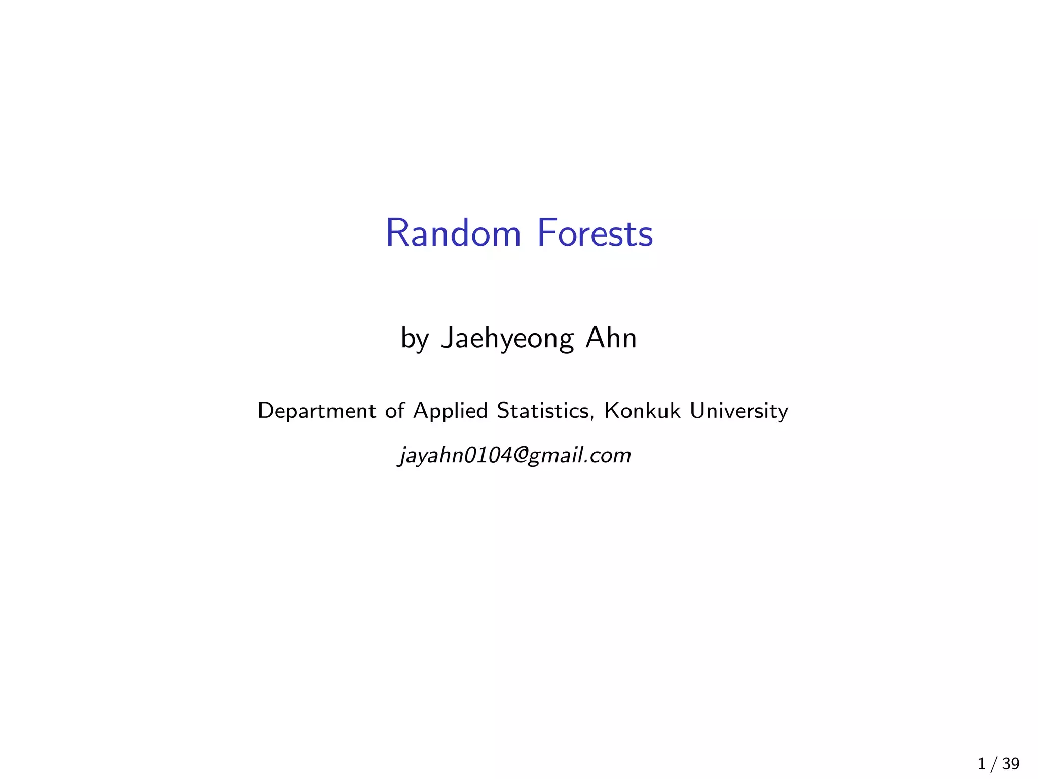
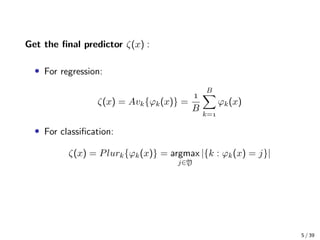
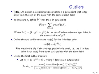
7. • Define an estimator of Eθϕ(x, θ)
AVkϕk(x) → Eθϕ(x, θ), (AVkϕk(x) = 
B
B
k= ϕ(x, θk))
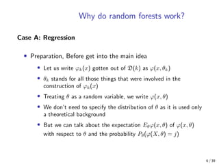
• Define the Prediction Error(risk) of the forest
PE∗
(forest) = E|Y − Eθϕ(Y, θ)|
, (E stands for EX,Y )
• Define the average(expected) Prediction Error of individual tree
PE∗
(tree) = EθE|Y − ϕ(X, θ)|
• Assume the Unbiasedness of forest and tree(strong assumption)
E[Y − Eθϕ(x, θ)] = , E[Y − ϕ(X, θ)] = , ∀θ
7 / 39

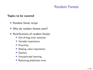
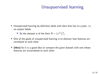
8. • Express PE∗
(forest) using Covariance
PE∗
(forest)= E|Y − Eθϕ(X, θ)|
= E|Eθ[Y − ϕ(X, θ)]|
, ( Y is independent from θ)
= E{Eθ[Y − ϕ(X, θ)] · Eθ [Y − ϕ(X, θ )]}
= EEθ,θ (Y − ϕ(X, θ)) · (Y − ϕ(X, θ ))
= Eθ,θ E(Y − ϕ(X, θ)) · (Y − ϕ(X, θ ))
= Eθ,θ Cov Y − ϕ(X, θ), Y − ϕ(X, θ )
Where θ, θ are independent with the same distribution
• Using the covariance-correlation formula
Cov Y − ϕ(x, θ), Y − ϕ(x, θ )
= ρ Y − ϕ(x, θ), Y − ϕ(x, θ ) · std (Y − ϕ(x, θ)) · std Y − ϕ(x, θ )
= ρ(θ, θ )sd(θ)sd(θ )
Where ρ(θ, θ ) is the correlation between Y − ϕ(x, θ) and Y − ϕ(x, θ ),
sd(θ) denotes the standard deviation of Y − ϕ(x, θ)
8 / 39

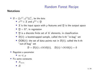
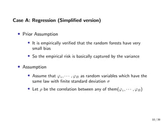
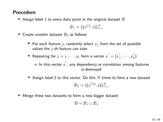
9. • Express PE∗
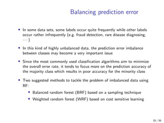
(forest) using correlation
PE∗
(forest) = Eθ,θ {ρ(θ, θ )sd(θ)sd(θ )}
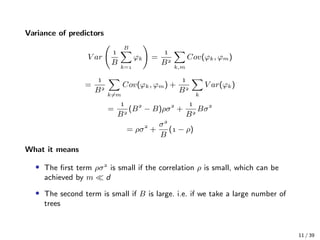
• Define the weighted average correlation ¯ρ
¯ρ =
Eθ,θ {ρ(θ, θ )sd(θ)sd(θ )}
Eθsd(θ)Eθ sd(θ )
• Show the inequality between PE∗
(forest) and PE∗
(tree) by the
property of Variance
PE∗
(forest) = ¯ρ(Eθsd(θ))
≤ ¯ρEθ(sd(θ))
= ¯ρEθE|Y − ϕ(X, θ)|
, ( E[Y − ϕ(X, θ)] = , ∀θ)
= ¯ρPE∗
(tree)
• What this inequality means
”the smaller the correlation, the smaller the prediction error.”
⇒ This shows why Random forest limits the number of variables m d
at each node
because it’s reasonable to assume that two sets of features that have not
much overlap between them should in general have a small correlation
9 / 39

10. Case A: Regression (Simplified version)
• Prior Assumption
• It is empirically verified that the random forests have very
small bias
• So the empirical risk is basically captured by the variance
• Assumption
• Assume that ϕ, · · · , ϕB as random variables which have the
same law with finite standard deviation σ
• Let ρ be the correlation between any of them(ϕ, · · · , ϕB)
10 / 39

11. Variance of predictors
V ar

B
B
k=
ϕk =

B
k,m
Cov(ϕk, ϕm)
=

B
k=m
Cov(ϕk, ϕm) +

B
k
V ar(ϕk)
=

B
(B
− B)ρσ
+

B
Bσ
= ρσ
+
σ
B
( − ρ)
What it means
• The first term ρσ
is small if the correlation ρ is small, which can be
achieved by m d
• The second term is small if B is large. i.e. if we take a large number of
trees
11 / 39

12. Case B: Classification
• Define the estimator of argmax
j
Pθ(ϕ(X, θ) = j)
argmax
j

B
|{k : ϕ(X, θk) = j}| → argmax
j
Pθ(ϕ(X, [theta) = j)
• Define the Margin Function
mr(X, Y ) = Pθ(ϕ(X, θ) = Y ) − max
j=Y
Pθ(ϕ(X, θ) = j)
• in the limit as k → ∞
• (i) if mr(X, Y ) ≥ , then the R.F classifier ζ will predict that
the class label of X is Y
• (ii) if mr(X, Y ) < , then the R.F classifier ζ will predict that
the class label of X is something other than Y
• Hence, the classification error occurs when and only when
mr(X, Y ) <  (ignore the tie case)
12 / 39

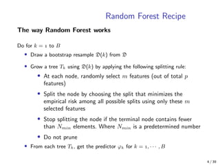
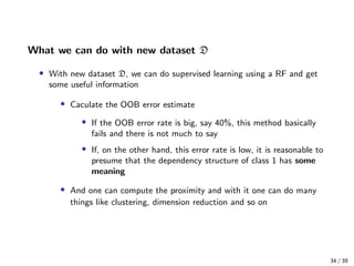
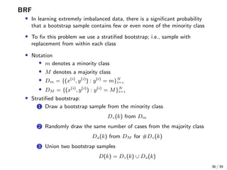
13. • Define the Prediction Error of forest classifier using mr(X, Y )
PE∗
= P(mr(X, Y ) < )
• Define the mean(expectation) s of mr(X, Y )
s = E[mr(X, Y )]
s represents the strength of the individual classifiers in the forest
• (Lemma 1) Let U be a random variable and let s be any positive
number. Then
Prob[U < ] ≤
E|U − s|
s
proof: by the Chebyshev inequality
• Express the inequality of Prediction Error by Lemma 1
PE∗
≤
V ar(mr)
s
, (assume s > )
13 / 39

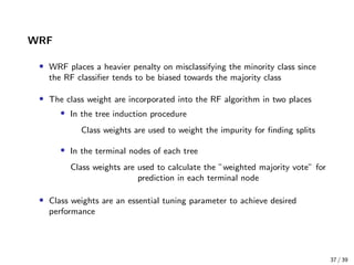
14. • Define ˆj(X, Y ) for simple notation
ˆj(X, Y ) = argmax
j=Y
Pθ(ϕ(x, θ) = j)
• Express mr(X, Y ) using ˆj(X, Y )
mr(X, Y )= Pθ[ϕ(X, θ) = Y ] − Pθ[ϕ(X, θ) = ˆj(X, Y )]
= Eθ[I(ϕ(X, θ) = Y ) − I(ϕ(X, θ) = ˆj(X, Y ))]
• Define rmg(θ, X, Y ) for simple notation
rmg(θ, X, Y ) = I(ϕ(X, θ) = Y ) − I(ϕ(X, θ) = ˆj(X, Y ))
• Hence we can express mr(X, Y ) using rmg(θ, X, Y )
mr(X, Y ) = Eθ[rmg(θ, X, Y )]
14 / 39

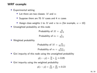
15. • Express V ar(mr) by Covariance
V ar(mr)
= E(Eθrmg(θ, X, Y ))
− (EEθrmg(θ, X, Y ))
= EEθrmg(θ, X, Y )Eθ rmg(θ , X, Y ) − EEθrmg(θ, X, Y )EEθ rmg(θ , X, Y )
= EEθ,θ {rmg(θ, X, Y )rmg(θ , X, Y )} − EθErmg(θ, X, Y )Eθ Ermg(θ , X, Y )
= Eθ,θ {E[rmg(θ, X, Y )rmg(θ , X, Y )] − Ermg(θ, X, Y )Ermg(θ , X, Y )}
= Eθ,θ Cov rmg(θ, X, Y ), rmg(θ , X, Y )
• Using the Covariance - Correlation formula
Cov rmg(θ, X, Y ), rmg(θ , X, Y )
= ρ rmg(θ, X, Y ), rmg(θ , X, Y ) · std(rmg(θ, X, Y ) · std(rmg(θ , X, Y ))
= ρ(θ, θ )sd(θ)sd(θ )
Where ρ(θ, θ ) is the correlation between rmg(θ, X, Y ) and rmg(θ , X, Y ),
sd(θ) is the standard deviation of rmg(θ, X, Y )
15 / 39

16. • Express V ar(mr) using correlation
V ar(mr) = Eθ,θ [ρ(θ, θ )sd(θ)sd(θ )]
• Define the weighted average correlation ¯ρ of rmg(θ, X, Y ) and
rmg(θ , X, Y )
¯ρ =
Eθ,θ [ρ(θ, θ )sd(θ)sd(θ )]
Eθ,θ [sd(θ)sd(θ )]
16 / 39

17. • Show the inequality of V ar(mr) using the fact that |¯ρ| ≤ 1 and
sd(θ) = sd(θ )
V ar(mr) = ¯ρ{Eθsd(θ)}
≤ ¯ρEθ[sd(θ)]
• Unfold Eθ[sd(θ)]
Eθ[sd(θ)]
= EθE[rmg(θ, X, Y )]
− Eθ[Ermg(θ, X, Y )]
• Show the inequality of s by ...
s = E(mr(X, Y )) = EEθrmg(θ, X, Y ) = EθErmg(θ, X, Y )
s
= {EθErmg(θ, X, Y )}
≤ Eθ[Ermg(θ, X, Y )]
• Therefore
Eθ[sd(θ)]
≤ EθE[rmg(θ, X, Y )]
− s
• Show the inequality of EθE[rmg(θ, X, Y )]
EθE[rmg(θ, X, Y )]
≤ 
( rmg(θ, X, Y ) = I(something) − I(somethingelse),
Which can only take 0 or ±1 for its value)
17 / 39

18. • Show the inequality of Prediction Error
PE∗
≤ ¯ρ
 − s
s
• Above inequality can be proven by the inequalities we’ve shown before
1
PE∗
≤
V ar(mr)
s
2
V ar(mr) = ¯ρ{Eθsd(θ)}
≤ ¯ρEθ[sd(θ)]
3
Eθ[sd(θ)]
≤ EθE[rmg(θ, X, Y )]
− s
4
EθE[rmg(θ, X, Y )]
≤ 
• What this inequality means
”the smaller the correlatoin, the smaller the prediction error”
18 / 39

19. Ramifications of RF
We now show how to exploit the RF to extract some important
side information
19 / 39

20. Out-of-Bag(OOB) error estimate
• Recall that at stage k, for k = , · · · , B, of the RF
construction, roughly 1/3 of D is left out from the bootstrap
sample D(k), and this left-out set is denoted by OOB(k)
• As we wrote before, D is a disjoint union of D(k) and OOB(k)
• For each k, using D(k), construct a tree Tk which a predictor
ϕk(x) is derived
• (Idea) Since OOB(k) is not used in the construction of
ϕk(x), it can be used to test ϕk(x)
⇒ So OOB error can be obtained as a proxy for the
generalization error
20 / 39

21. Procedure
• For each data point x(i)
∈ OOB(k), compute ϕk(x(i)
) only if x(i)
is in
OOB(k) for all k = , · · · , B
• Aggregate the OOB predictors ϕk(x(i)
) for only some k = , · · · , B.
Since we only consider the OOB sets which have x(i)
• For regression:
α(x(i)
) = Avk{ϕk(x(i)
)}
• For classification:
α(x(i)
) = Plurk{ϕk(x(i)
)}
• To compute α(x(i)
) for all i = , · · · , N B must be big enough
• Since the probability of any single data point belonging in all of
D(k) for k = , · · · , B is very small if B is big enough
• Obtain the overall error(OOB error estimate) of the random forest
OOBerror = {x(i)∈OOB(k)}B

L(yi, α(x(i)
)
• In regression: L(yi, α(x(i)
) denotes a square loss function
• In classification: L(yi, α(x(i)
)) denotes a misclassification error
⇒ We may regard OOBerror as a reasonably good proxy for the generalization
error
21 / 39

22. Variable importance
Impurity importance
• Recall that in the RF recipe at each node the split decision is made to
make the impurity(empirical risk) decrease the most
• (Idea) At that node, it is reasonable to presume the variable involved
with the split decision is the most important one
• The impurity importance of each variable is the addition of the absolute
values of such decrease amounts for all splits in all trees in the forest
every time the split is done using that variable
• Notations
• Tj is the set of all nodes split by j-th variable
• ∆Rnt denotes the decrease amounts of empirical risk at node t
• Define the impurity variable importance of j-th feature
V I(j) =
t∈Tj
|∆Rnt|
22 / 39

23. Permutation importance
• The permutation importance assumes that the data value associated with
an important variable must have a certain structural relevance to the
problem
• (Idea) So that the effect of a random shuffling (permutation) of its data
value must be reflected in the decrease in accuracy of the resulting
predictor
• Notations
• D = {x()
, · · · , x(n)
}
• x(i)
= [x
(i)
 , · · · , x
(i)
p ]T
• Write D in matrix form
D =








x · · · xj · · · xp
...
...
...
xi · · · xij · · · xip
...
...
...
xn · · · xnj · · · xnp








in which xij = x
(i)
j for all i = , · · · , n and j = , · · · , p
23 / 39

24. • Let π be a permutation on {, · · · , n} denoted by
π =
1 2 · · · n
π(1) π(2) · · · π(n)
• Define the permuted data set D(π, j) gotten from D by applying π to the
j-th column
D(π, j) =








x · · · xπ()j · · · xp
...
...
...
xi · · · xπ(i)j · · · xip
...
...
...
xn · · · xπ(n)j · · · xnp








⇒In D(π, j) the values of the j-th column in D is shuffled by the
permutation π
• So, if xj is important, the error using the randomly shuffled dataset
D(π, j) should be much worse that that using the correct dataset D
• On the other hand, a variable has not much relevance or importance, if
the error using D(π, j) is more or less the same as the one with D
24 / 39

25. Permutation importance by OOB set
Classification
• For each k, let ϕk be the predictor associated with the tree Tk
Let πk be a permutation on the k-th out-of-bag set OOB(k)
• Define C(π, j, k)
C(π, j, k) =
(x(i),y(i))∈OOB(k)
I y(i)
= ϕk(x(i)
) − I y(i)
= ϕk(x(i)
(πk, j))
• Define the permutation variable importance of the j-th variable xj in k-th
tree
V I(j, k) =
C(πk, j, k)
|OOB(k)|
• Define the permutation variable importance of the j-th variable xj in
forest
V I(j) =

B
B
k=
V I(j, k)
⇒ It is very reasonable to presume that the higher V I(j) is, the more
important xj is
25 / 39

26. Regression
• For each k, let ϕk be the regressor associated with the tree Tk
Let πk be a permutation on the k-th out-of-bag set OOB(k)
• Define S(k) which denotes the empirical risk of OOB set with square loss
S(k) =
(x(i),y(i))∈OOB(k)
|y(i)
− ϕk(x(i)
)|
• Define S(π, j, k) which is the empirical risk of the permuted OOB set in
which x(i)
is replaced with x(i)
(πk, j)
S(π, j, k) =
(x(i),y(i))∈OOB(k)
|y(i)
− ϕk(x(i)
(πk, j))|
• Define the permutation variable importance of the j-th variable xj in k-th
tree
V I(j, k) =
S(πk, j, k)
S(k)
• Define the permutation variable importance of the j-th variable xj in
forest
V I(j) =

B
B
k=
V I(j, k)
⇒the higher V I(j) is, the more important xj is
26 / 39

27. Proximity
• The proximity of two data points is as measure of how close they are
• Knowledge of the proximity for all data points, if available, is very
important information that can be exploited in many ways (e.g. nonlinear
dimension reduction, clustering problems, · · · )
• However defining the proximity of categorical varaible is some what
challenging. And also in numeric data, normalizing the unit of
measurement is not that simple issue (e.g. meters, millimeters,
kilometers, · · · )
• RF provides a handy and sensible way of defining the proximity
• RF defines the proximity of two data points using terminal nodes
• (Idea) If two data points end up in the same terminal node, then they are
close (the proximity is 1)
27 / 39

28. • Recall that RF constructs a tree Tk for each bootstrap sample D(k) for
k = , · · · , B. And from Tk, k-th predictor ϕk is derived
• Let vk(x) be the terminal node of x in k-th tree Tk
• Given any input x, one can put it down the tree Tk to eventually
arrive at a terminal node which is denoted by vk(x)
• Two input points with the same terminal nodes have the same ϕk(x)
values but the converse does not hold
• Define the k-th proximity Proxk(i, j) of two data points x(i)
and x(j)
,
regardless of whether in-bag or out-of-bag for each k = , · · · , B, and for
i, j = , · · · , N
Proxk(i, j) =
 if vk(x(i)
) = vk(x(j)
)
 if vk(x(i)
) = vk(x(j)
)
⇒ this says that Proxk(i, j) =  if and only if x(i)
and x(j)
end up in the
same terminal node after the tree run on Tk
• Define the Proximity of forest
Prox(i, j) =

B
B
k=
Proxk(i, j)
• Note that Prox(i, i) =  and  < Prox(i, j) ≤  28 / 39

29. Missing value imputation
• Mean/mode replacement (rough fill)
This is a fast and easy way to replace missing values
• If xj is numeric, then take as the imputed value the mean or
median of the non-missing vlaues of the j-th feature
• If xj is categorical, then take the most frequent value
(majority vote) of the j-th feature
29 / 39

30. • Proximity-based imputation
1 Do a rough fill (mean/mode imputation) for missing input values
2 Construct a RF with the imputed input data and compute the
proximity using this RF
3 Let xij = x
(i)
j be a missing value in the original dataset (before any
imputation)
• Case A: xij is numerical
Take the weighted average of the non-missing vlaues weighted
by the proximity
xij =
k∈Nj
Prox(i, k)xkj
k∈Nj
Prox(i, k)
,
where Nj = {k : xkj is non-missing}
• Case B: xij is categorical
Replace xij with the most frequent value where the frequency
is calculated with the proximity as weights
xij = argmax {
k∈Nj
Prox(i, k)I(xkj = )}
4 Repeat (2), (3) several times (typically 4 ∼ 6 times)
30 / 39

31. Outliers
• (Idea) An outlier in a classification problem is a data point that is far
away from the rest of the data with the same output label
• To measure it, define ¯P(i) for the i-th data point
¯P(i) =
k∈L(i)
Prox
(i, k),
Where L(i) = {k : y(k)
= y(i)
} is the set of indices whose output label is
the same as that of y(i)
• Define the raw outlier measure mo(i) for the i-th data point
mo(i) = N/ ¯P(i)
This measure is big if the average proximity is small, i.e. the i-th data
point is far away from other data points with the same label
• Define the final outlier measure
• Let N = {i : y(i)
= } , where denotes an output label
fmo(i) =
mo(i) − median (mo(i)I(i ∈ N ))N

i∈N ((mo(i) − median(mo(i)I(i ∈ N ))N
 )
31 / 39

32. Unsupuervised learning
• Unsupervised learning by definition deals with data that has no y-part, i.e.
no output labels.
• So the dataset is of the form D = {x(i)
}N
i=
• One of the goals of unsupervised learning is to discover how features are
correlated to each other
• (Idea) So it is a good idea to compare the given dataset with one whose
features are uncorrelated to each other
32 / 39

33. Procedure
• Assign label 1 to every data point in the original dataset D
D = {(x(i)
, )}N
i=
• Create anotehr dataset D2 as follows
• For each feature j, randomly select xj from the set of possible
values the j-th feature can take
• Repeating for j = , · · · , p, form a vector x = (x, · · · , xp)
⇒ In this vector x , any dependency or correlation among features
is destroyed
• Assign label 2 to this vector. Do this N times to form a new dataset
D = {(x (i)
, )}N
i=
• Merge these two datasets to form a new bigger dataset
D = D ∪ D
33 / 39

34. What we can do with new dataset D
• With new dataset D, we can do supervised learning using a RF and get
some useful information
• Caculate the OOB error estimate
• If the OOB error rate is big, say 40%, this method basically
fails and there is not much to say
• If, on the other hand, this error rate is low, it is reasonable to
presume that the dependency structure of class 1 has some
meaning
• And one can compute the proximity and with it one can do many
things like clustering, dimension reduction and so on
34 / 39

35. Balancing prediction error
• In some data sets, some labels occur quite frequently while other labels
occur rather infrequently (e.g. fraud detection, rare disease diagnosing,
· · · )
• In this kind of highly unbalanced data, the prediction error imbalance
between classes may become a very important issue
• Since the most commonly used classification algorithms aim to minimize
the overall error rate, it tends to focus more on the prediction accuracy of
the majority class which results in poor accuracy for the minority class
• Two suggested methods to tackle the problem of imbalanced data using
RF:
• Balanced random forest (BRF) based on a sampling technique
• Weighted random forest (WRF) based on cost sensitive learning
35 / 39

36. BRF
• In learning extremely imbalanced data, there is a significant probability
that a bootstrap sample contains few or even none of the minority class
• To fix this problem we use a stratified bootstrap; i.e., sample with
replacement from within each class
• Notation
• m denotes a minority class
• M denotes a majority class
• Dm = {(x(i)
, y(i)
) : y(i)
= m}N
i=
• DM = {(x(i)
, y(i)
) : y(i)
= M}N
i=
• Stratified bootstrap:
1 Draw a bootstrap sample from the minority class
D(k) from Dm
2 Randomly draw the same number of cases from the majority class
D(k) from DM for #D(k)
3 Union two bootstrap samples
D(k) = D(k) ∪ D(k)
36 / 39

37. WRF
• WRF places a heavier penalty on misclassifying the minority class since
the RF classifier tends to be biased towards the majority class
• The class weight are incorporated into the RF algorithm in two places
• In the tree induction procedure
Class weights are used to weight the impurity for finding splits
• In the terminal nodes of each tree
Class weights are used to calculate the ”weighted majority vote” for
prediction in each terminal node
• Class weights are an essential tuning parameter to achieve desired
performance
37 / 39

38. WRF example
• Experimental setting
• Let there are two classes: M and m
• Suppose there are 70 M cases and 4 m cases
• Assign class weights 1 to M and w to m (for example, w = 10)
• Unweighted probability at this node
Probability of M = 70
70+4
Probability of m = 4
70+4
• Weighted probability
Probability of M = 70
70+4∗w
Probability of m = 4∗w
70+4∗w
• Gini impurity of this node using the unweighted probability
p( − p) = 70
74
∗ 4
74
≈ 0.05
• Gini impurity using the weighted probability
p( − p) = 70
110
∗ 40
110
≈ 0.23
38 / 39

39. References
1 Breiman, Leo. ”Random forests.” Machine learning 45, no. 1 (2001):
5-32.
2 Breiman, L. and Cutler, A., Random Forests,
https://www.stat.berkeley.edu/∼breiman/RandomForests/cc home.htm
3 Hyeongin Choi, Lecture 10: Random Forests,
http://www.math.snu.ac.kr/ hichoi/machinelearning/lecturenotes/Ran-
domForests.pdf
4 Chen, Chao Breiman, Leo. (2004). Using Random Forest to Learn
Imbalanced Data. University of California, Berkeley.
https://statistics.berkeley.edu/sites/default/files/tech-reports/666.pdf
39 / 39