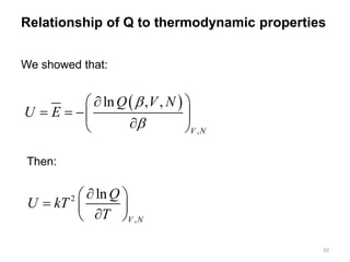
1) The document describes the canonical partition function for an ideal monatomic gas. It shows that the partition function can be broken into translational, electronic, and nuclear contributions which are independent. 2) Key relationships are developed between the partition function and thermodynamic properties like internal energy, entropy, heat capacity, and more. Knowing the partition function provides expressions for properties like the Helmholtz free energy. 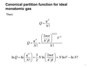3) For an ideal monatomic gas, the translational partition function is derived and shown to be proportional to volume to the power of 3/2. The electronic and nuclear contributions are accounted for but not explicitly derived.

1. The Ideal Monatomic
Gas

2. Canonical ensemble: N, V, T
2

3. Canonical partition function for ideal monatomic gas
A system of N non-interacting identical atoms:
!
N
q
Q
N

states i energy levels
of a single atom
j
i
j
q e e





 
 
   
2
2 2 2
2 3
, ,
8
x y z x y z
h
l l l l l l
mV
   
From quantum mechanics:
Atom of ideal gas in cubic box
of volume V
3

4. Canonical partition function for ideal monatomic gas
Translational quantum numbers
, , :
x y z
l l l
 
2 2 2 2
2 3
2 2
2 2 2 2
2 3 2 3 2 3
8
states i
8 8 8
x y z
i
x y z
y
x z
x y z
h l l l
mV
l l l
h l
h l h l
mV mV mV
x y z
l l l
q e e
e e e q q q



 
 


  
  
 
   
 
    
 
  
 
  
 
  
4

5. With suitable assumptions:
3 2
2
2m
q V
h


 
  
 
• Approximate each sum and solve as an
integral
• Then compute q
• Then compute Q
5

6. The calculated Q is the canonical partition
function for ideal monatomic gas
We have considered the contribution of atomic translation to
the partition function
However, we have not included other effects, such as
contribution of the electronic and nuclear energy states.
We will get back to this matter later in this slide set.
6

7. Canonical partition function for ideal
monatomic gas
Then:
!
N
q
Q
N

3 2
2
2
! !
N
N
N
m
V
h
q
Q
N N


 
 
 
 
2
3 2
ln ln ln ln ln !
! 2
N
q m
Q N N V N
N h


   
   
   
 
 
7

8. Canonical partition function for ideal monatomic gas
The internal energy of a N-particle monatomic ideal gas is:
,
ln 3
2
V N
Q N
U
 
 

  
 

 
But U of a monatomic ideal gas is known to be:
,
ln 3
2
V N
Q
U NkT

 

  
 

 
8

9. Canonical partition function for ideal monatomic gas
Then:
1
kT
 
Note that is only a function of the thermal reservoir,
regardless of the system details. Therefore, this
identification is valid for any system.

9

10. Relationship of Q to thermodynamic properties
Then:
We showed that:
 
,
ln , ,
V N
Q V N
U E



 
   

 
2
,
ln
V N
Q
U kT
T

 
  

 
10

11. Relationship of Q to thermodynamic properties
Multiplying by kT2:
For a system with fixed number of particles N:
, ,
ln ln
ln
V N T N
Q Q
d Q dT dV
T V
 
   
 
   
 
   
2 2 2
, ,
ln ln
ln
V N T N
Q Q
kT d Q kT dT kT dV
T V
 
   
 
   
 
   
2 2
,
ln
ln
T N
Q
kT d Q UdT kT dV
V

 
   

  11

12. Relationship of Q to thermodynamic properties
Combining:
But: 2
2
1
U U U
d dU dT UdT T d TdU
T T T T
   
     
   
   
dV
V
Q
kT
Q
d
kT
T
U
d
T
TdU
dV
V
Q
kT
Q
d
kT
T
U
d
T
TdU
dV
V
Q
kT
Q
d
kT
UdT
T
U
d
T
dT
T
Q
kT
TdU
T
U
d
T
UdT
TdU
N
T
N
T
N
T
N
V
,
2
2
2
,
2
2
2
,
2
2
2
,
2
2
ln
ln
ln
ln
ln
ln
ln




































































12

13. Therefore:
,
, ,
ln
ln
ln ln
ln
T N
V N T N
U Q
dU kTd Q kT dV
kT V
Q Q
kTd Q T kT dV
T V

   
   
   

   
 
 
   
 
 
   
 
 
   
 
13

14. Relationship of Q to thermodynamic properties
We identify that:
Comparing this result with:
dU TdS PdV
 
,
,
ln
ln
ln
T N
V N
Q
P kT
V
Q
dS kd Q T
T

 
  

 
 

 
 
 
 
 

 
 
14

15. Relationship of Q to thermodynamic properties
The entropy:
,
ln
ln
V N
Q
S Q T
T

 
   

 
The Helmholtz free energy:
   
, , ln , ,
A T V N kT Q T V N
 
2
, ,
ln ln
ln
V N V N
Q Q
A U TS kT kT Q T
T T
   
 
   
    
   
   
   
 
   
   
15

16. Relationship of Q to thermodynamic properties
The Helmholtz energy:
   
, , ln , ,
A T V N kT Q T V N
 
This is a very important equation – knowing the canonical
partition function is equivalent to having an expression for
the Helmholtz energy as function of temperature, volume
and number of molecules (or moles). From such
expression, it is possible to derive any thermodynamic
property
16

17. Relationship of Q to thermodynamic properties
The chemical potential of a pure substance:
The enthalpy:
   
, ,
, , ln , ,
T V T V
A T V N Q T V N
kT
N N

 
   
  
   
 
   
2
, ,
ln ln
V N T N
Q Q
H U PV kT kTV
T V
 
   
   
   
 
   
17

18. Relationship of Q to thermodynamic properties
Heat capacity at constant volume:
2
,
,
,
2
2
2
, ,
ln
ln ln
2
V N
V
V N
V N
V N V N
Q
kT
T
U
C
T T
Q Q
kT kT
T T
 
 

 

 
 
 

 

   
 
  
   
 
 
 
 
 
 
 
 
  
 
 
   
18

19. Relationship of Q to thermodynamic properties
The previous expression can also be written as:
2
2 2 2
2 2
, ,
,
2
V
V N V N
V N
kT Q kT Q kT Q
C
Q T Q T Q T
 
  
   
  
 
   
  
   
 
This form will be useful when discussing fluctuations, later
in this slide set
19

20. Thermodynamic properties of monatomic ideal
gases
The previous slides showed how to evaluate thermodynamic
properties given Q
It is time to discuss the effect of the electronic and nuclear
energy states to the single atom partition function before
proceeding with additional derivations
We will assume the Born-Oppenheimer approximation:
translational energy states are independent of the electronic
and nuclear states
Besides, we will assume the electronic and nuclear states are
independent of each other
20

21. Thermodynamic properties of monatomic ideal
gases
With these assumptions:
trans elec nuc
   
  
The single atom partition function is:
 
states of the atom
trans elec nuc
kT
q e
  
 

 
As discussed in the previous class for independent energy
modes:
trans elec nuc
q q q q

21

22. Thermodynamic properties of monoatomic ideal gases
In which:
,
translational states i
trans i
kT
trans
q e


 
,
electronic states i
elec i
kT
elec
q e


 
,
nuclear states i
nuc i
kT
nuc
q e


 
22

23. Thermodynamic properties of monatomic ideal
gases
3 2 3 2
2 2
2 2
trans
m m kT
q V V
h h
 

   
   
 
 
 
3
trans
V
q 

2
2
h
m kT

 
   
 
 De Broglie wavelength: based on dual
wave-particle nature of matter
23

24. Thermodynamic properties of monatomic ideal
gases
The electronic partition function:
 
,
,
,1 ,2 ,3
,2 ,1 ,3
,1
,
electronic states i electronic levels j
,1 ,2 ,3
,1 ,2 ,3
...
elec j
elec i
elec elec elec
elec elec elec
elec
kT kT
elec elec j
kT kT kT
elec elec elec
kT kT
elec elec elec
q e e
e e e
e e e


  
  


  
  
 
  

  
  
   
 
 
 
,1
,1 ,2 ,3
,1 ,2 ,3
...
...
elec
elec elec elec
kT
kT kT kT
elec elec elec
e e e

  
  

 
  
 
 
 
 
 
 
  
 
 
  24

25. Thermodynamic properties of monatomic ideal
gases
The electronic partition function:
,1 ,2 ,3
,1 ,2 ,3 ...
elec elec elec
kT kT kT
elec elec elec elec
q e e e
  
  
 
  
 
   
 
 
 
Additional information and approximations:
-The degeneracy of the ground energy level is equal to 1 in
noble gases, 2 in alkali metals, 3 in Oxygen;
-The ground energy level is the reference for the
calculations – it is conventional to set it to zero;
-The differences in electronic levels are high. For example,
argon:
,2 1521
elec
kJ
mol

  At room T:
,2
450
0
elec
kT
e e




  25

26. Thermodynamic properties of monatomic ideal
gases
Then, the electronic partition function is approximated as:
,1
elec elec
q 

26

27. Thermodynamic properties of monatomic ideal
gases
The nuclear partition function:
The analysis is similar to that of the electronic partition function,
only that the energy levels are even farther apart.
It results:
,1
nuc nuc
q 

Also, in situations of common interest to chemical engineers,
the atomic nucleus remains largely undisturbed. The nuclear
partition function becomes only a multiplicative factor that will
cancel out in calculations
27

28. Thermodynamic properties of monatomic ideal
gases
Compiling all these intermediate results:
trans elec nuc
q q q q

3 2
,1 ,1 2
2
elec nuc
m kT
q V
h

 
 
  
 
3 2
,1 ,1 2
2
! !
N
elec nuc
N
m kT
V
h
q
Q
N N

 
 
 
 
 
 
 
 
 
28

29. Thermodynamic properties of monatomic ideal
gases
For the monoatomic ideal gas, the logarithm of the
canonical partition function is:
3 2
,1 ,1 2
,1 ,1 2
2
ln ln ln
! !
3 2
ln ln ln ln ln !
2
N
elec nuc
N
elec nuc
m kT
V
h
q
Q
N N
m kT
N N N N V N
h

 

 
 
 
 
 
 
 
   
  
 
 
 
   
 
 
29

30. Thermodynamic properties of monatomic ideal
gases
Let us now use this expression to compute several
properties, beginning with the pressure:
,
ln
T N
Q NkT
P kT
V V

 
 
 

  Av
R
k
N

Av Av
NkT NRT NRT
P PV
V N V N
   
where N is the number of molecules and Nav is Avogadro’s
number.
30

31. Thermodynamic properties of monatomic ideal
gases
PV nRT

31

32. Thermodynamic properties of monatomic ideal
gases
PV nRT

We derived this very famous equation from very
fundamental principles – an amazing result
32

33. Thermodynamic properties of monatomic ideal
gases
Internal energy and heat capacity at constant volume:
2
,
ln
V N
Q
U kT
T

 
  

 
,1 ,1 2
3 2
ln ln ln ln ln ln !
2
elec nuc
m kT
Q N N N N V N
h

 
 
    
 
 
2 3 3
2 2
N
U kT NkT
T
 
,
3
2
V
V N
U
C Nk
T

 
 
 

 
These expressions are more complicated if excited energy
levels are taken into account – see eq. 3.4.12 and Problem
3.2 33

34. Thermodynamic properties of monatomic ideal
gases
Helmholtz energy:
Before obtaining its expression, let us introduce Stirling’s
approximation:
ln ! ln ln ln
N N N N N N N e
   
This approximation is increasingly accurate the larger N is. Since
N here represents the number of atoms, it is typically a very large
number and this approximation is excellent.
34

35. Thermodynamic properties of monatomic ideal
gases
Helmholtz energy:
3
2
,1 ,1
2
2
ln ln elec nuc
Ve
m kT
A kT Q NkT
h N
 

 
 
 
     
 
 
 
Ignoring the nuclear partition function by setting it equal to
1:
3
2
,1
2
2
ln ln elec
Ve
m kT
A kT Q NkT
h N


 
 
 
     
 
 
 
35

36. Thermodynamic properties of monatomic ideal
gases
Entropy:
U A
A U TS S
T

   
5
3
2
2
,1
2
2
ln elec
Ve
m kT
S Nk
h N


 
 
 
  
 
 
 
 
known as Sackur-Tetrode equation 36

37. Thermodynamic properties of monatomic ideal
gases
Chemical potential:
 
,
ln , ,
T V
Q T V N
kT
N


 
   

 
37

38. Thermodynamic properties of monatomic ideal gases
,1 ,1 2
,
,1 2
3 3
2 2
,1 ,1
2 2
3 2
ln ln ln ln ln
2
3 2
ln ln ln ln
2
2 2
ln ln
elec nuc
T V
elec
elec elec
m kT
N N N N V N N N
h
kT
N
m kT
kT V N
h
m kT V m kT kT
kT kT
h N h P

 



 
 
 
 
 
     
 
 
 
 
 
 
  
 

 
 
 
 
    
 
 
 
 
   
   
  
  
   
  
   
   
3
2
,1 2
0 0
3
2
,1 2
0 0
2
ln ln ln
2
ln ln
elec
elec
m kT kT kT kT
kT kT kT
h P P P
m kT kT P
kT kT
h P P




 

     
 
 
   
   
 
 
     
 
   
 
 
   
 
 
   
 
38

39. Thermodynamic properties of monatomic ideal
gases
Now compare this formula and the formula well-known to
chemical engineers of the chemical potential of a pure
ideal gas:
   
0
0
, , ln
P
T P T P kT
P
 
 
3
2
,1 2
0 0
2
ln ln
elec
m kT kT P
kT kT
h P P

 
 
 
 
  
 
 
 
 
39

40. Energy fluctuations in the canonical ensemble
In the canonical ensemble, the temperature, volume, and
number of molecules are fixed.
The energy may fluctuate. Assume its fluctuations follow a
Gaussian distribution:
 
2
1
2
1
2
x x
f x e

 
 

  
 
 

x 
Mean of the distribution Standard deviation
x  
f x
Variable Probability density
40

41. Energy fluctuations in the canonical ensemble
Given this distribution, the average value of any function
G(x) is calculated as follows:
     
2
1
2
1
2
x x
G f x G x dx e G x dx

 
 

    
 
 
 
 
 
The variance (standard deviation to power 2) is:
41
   
2 2 2 2
2 2 2 2
2 2
x x x xx x x xx x x x
          
 2
x  2
x  2
x  2
x

42. Energy fluctuations in the canonical ensemble
Let us apply this formalism to the average energy and its
fluctuation:
3
3
2
2
E
E U NkT x
NkT
   
3
2
E
x
NkT

 
2 2
2 2 2
2
1
3
2
x x E E
NkT
    
 
 
 
42
 2
E  2
E

43. Energy fluctuations in the canonical ensemble
 
2 2
2 2 2
2
1
3
2
x x E E
NkT
    
 
 
 
2
2
states i
2 states i
2 2
1
3
2
i
i
E
E
kT
kT
i
i
E e
E e
Q Q
NkT



 
 
 
 
 
 
 
 
   
   
   


43

44. 44
 
N
V
N
V
j
kT
E
j
j
kT
E
j
N
V
N
V
N
V
N
V
N
V
N
V
N
V
N
V
N
V
j
kT
E
j
N
V
N
V
j
kT
E
j
N
V
N
V
j
kT
E
j
j
kT
E
T
Q
Q
kT
T
Q
kT
Q
kT
Q
e
E
and
e
E
QkT
T
Q
Q
E
T
Q
Q
kT
T
Q
Q
kT
T
Q
Q
kT
Then
T
Q
Q
kT
T
Q
Q
kT
T
Q
Q
kT
T
E
T
Q
Q
kT
T
Q
kT
E
Since
e
E
QkT
T
Q
Q
E
T
E
e
kT
E
T
Q
E
Q
T
E
e
E
e
E
j
j
j
j
j
j
,
2
2
2
2
,
2
/
2
/
2
2
,
2
,
2
2
,
2
2
2
,
2
,
2
2
,
2
2
2
,
,
2
,
2
/
2
2
,
,
/
2
2
,
,
/
/
)
(
2
1
2
2
ln
1









































































































































































45. Energy fluctuations in the canonical ensemble
     
2 2
2
2 2 2
2
2
2 2 2
, ,
,
1
2
3
2
V N V N
V N
kT kT
kT T
Q Q Q
Q T Q T Q T
NkT

 
 
  
   
 
  
     
 
  
   
   
 
 
 
2
2 2 2
2 2
, ,
,
2
V
V N V N
V N
kT Q kT Q kT Q
C
Q T Q T Q T
 
  
   
  
 
   
  
   
 
We previously found that:
45

46. Energy fluctuations in the canonical ensemble
The 2/3 factor is a particularity of using monoatomic ideal
gases as example. However, the factor is common
and shows that relative fluctuations decrease as the
number of molecules increases.
Comparing these two expressions:
2
2
2
2 2
3
2 1
2
3
3 3
2 2
V
kT Nk
kT C
N
NkT NkT

 
 
 
   
   
   
   
2 1
3 N
  
1 N
46

47. Energy fluctuations in the canonical ensemble
47
d = [E/(3NkT/2)]-1

48. Gibbs entropy equation
But, using relationships developed in previous slides:
,
ln
ln
V N
Q
S Q T
T

 
   

 
2
, ,
states j
2
states j
,
ln 1
1 1
j
j
V N V N
E
kT
E
j
kT
V N
U Q Q
kT T Q T
e
E
e
Q T Q kT


 
   
  
   
 
   
 

 
  
 

 
 
 


48

49. Gibbs entropy equation
   
 
 
 
 
 
states j
states j
states j
, , ln , ,
ln ln , ,
, ,
1
ln , ,
, ,
ln , ,
j j
j
j j
E E
kT kT
E
kT
j
p N V E p N V E
e e Q N V T
Q N V T
E e
Q N V T
kT Q N V T
U
Q N V T
kT
 


 

 
 
  
  
 



49
Q
T
Q
T ln
ln












50. Gibbs entropy equation
Combining the expressions developed in the two previous
slides (algebra omitted here):
50
)
,
,
(
ln
)
,
,
(
ln
ln
,
j
statesj
j
N
V
E
V
N
p
E
V
N
p
k
T
Q
T
Q
k
S






















51. Gibbs entropy equation
If there is only one possible state:
   
states j
, , ln , , 1 ln1 0
j j
S k p N V E p N V E k
      

If there are only two possible states, assumed to have
equal probability:
   
states j
1 1 1 1
, , ln , , ln ln 0.693
2 2 2 2
j j
S k p N V E p N V E k k
 
   
      
   
 
   
 

If there are only three possible states, assumed to have
equal probability:
1 1 1 1 1 1
ln ln ln 1.0986
3 3 3 3 3 3
S k k
 
     
     
     
 
     
 
51