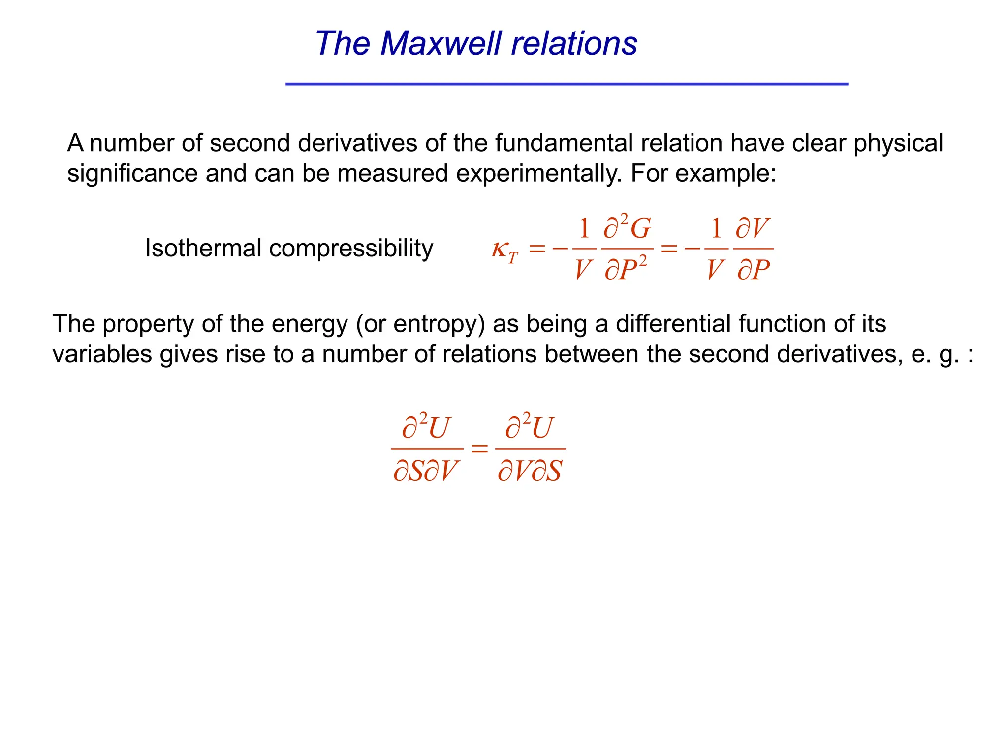
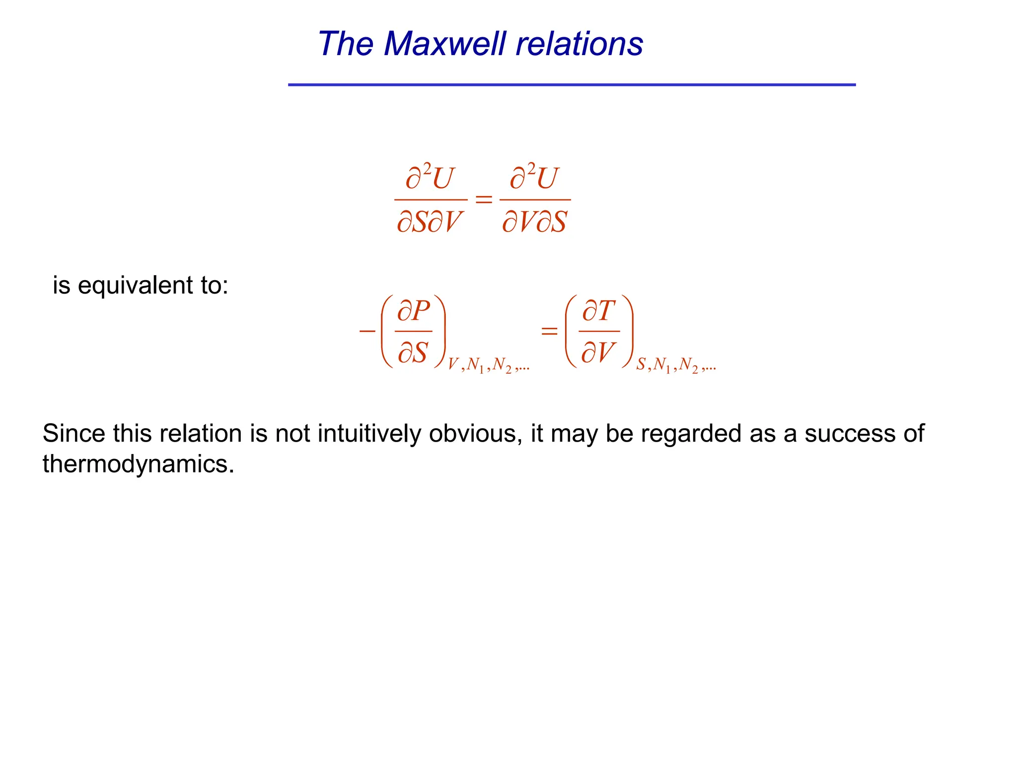
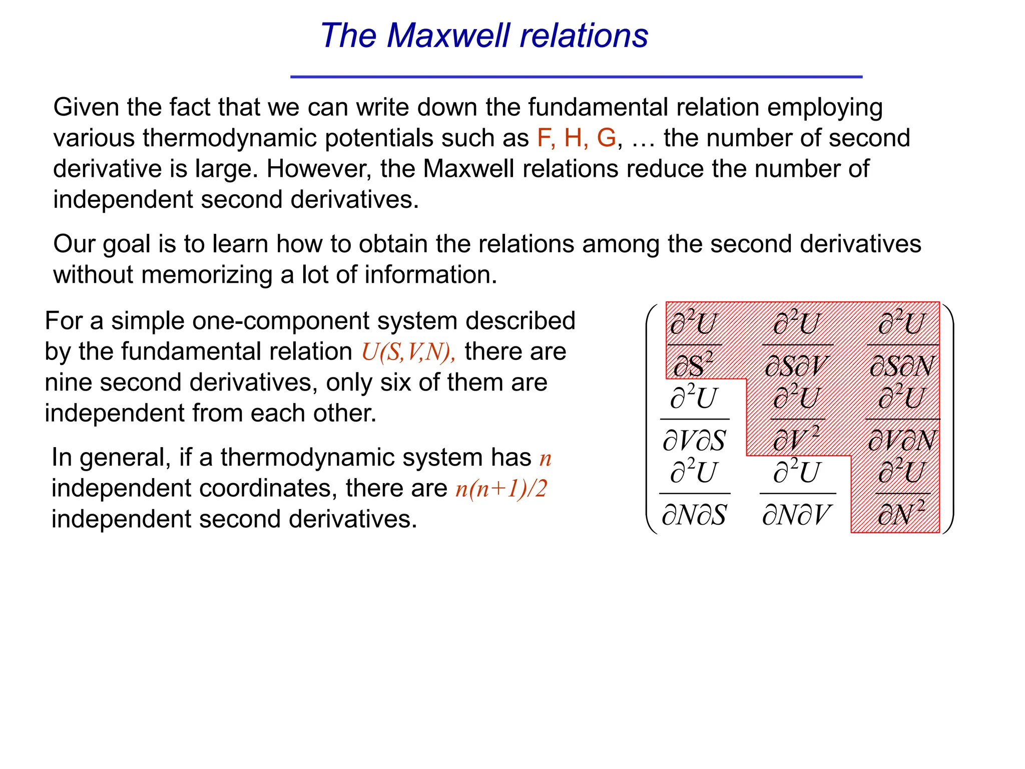
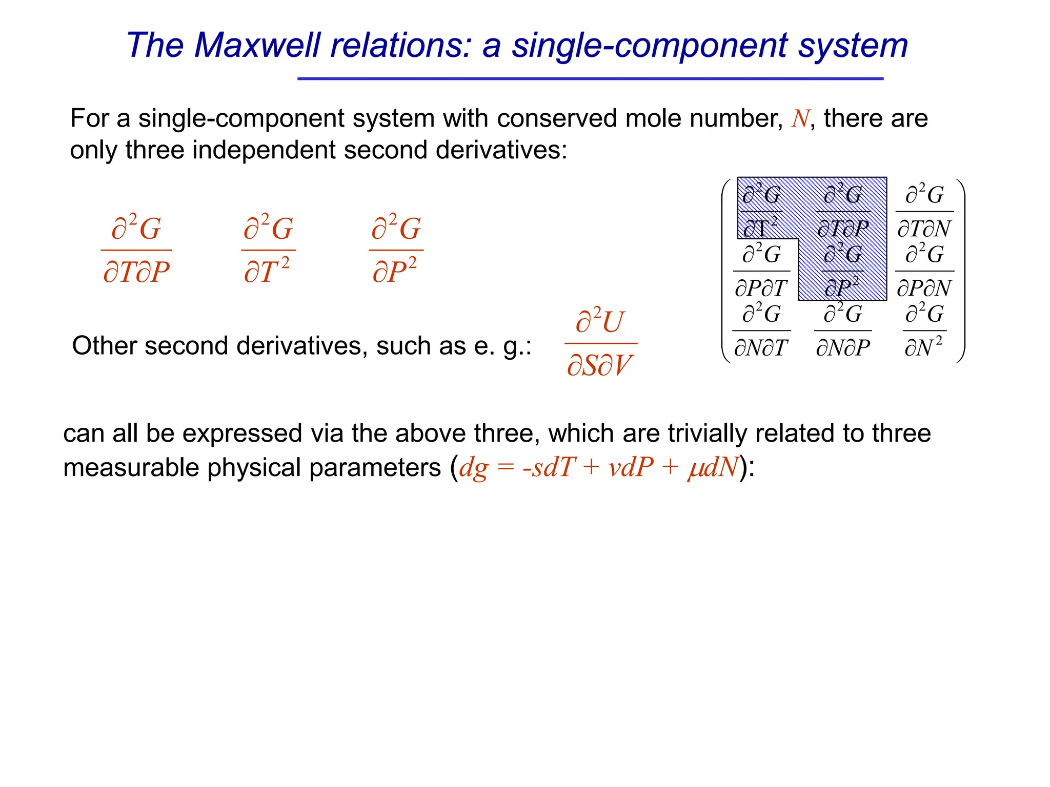
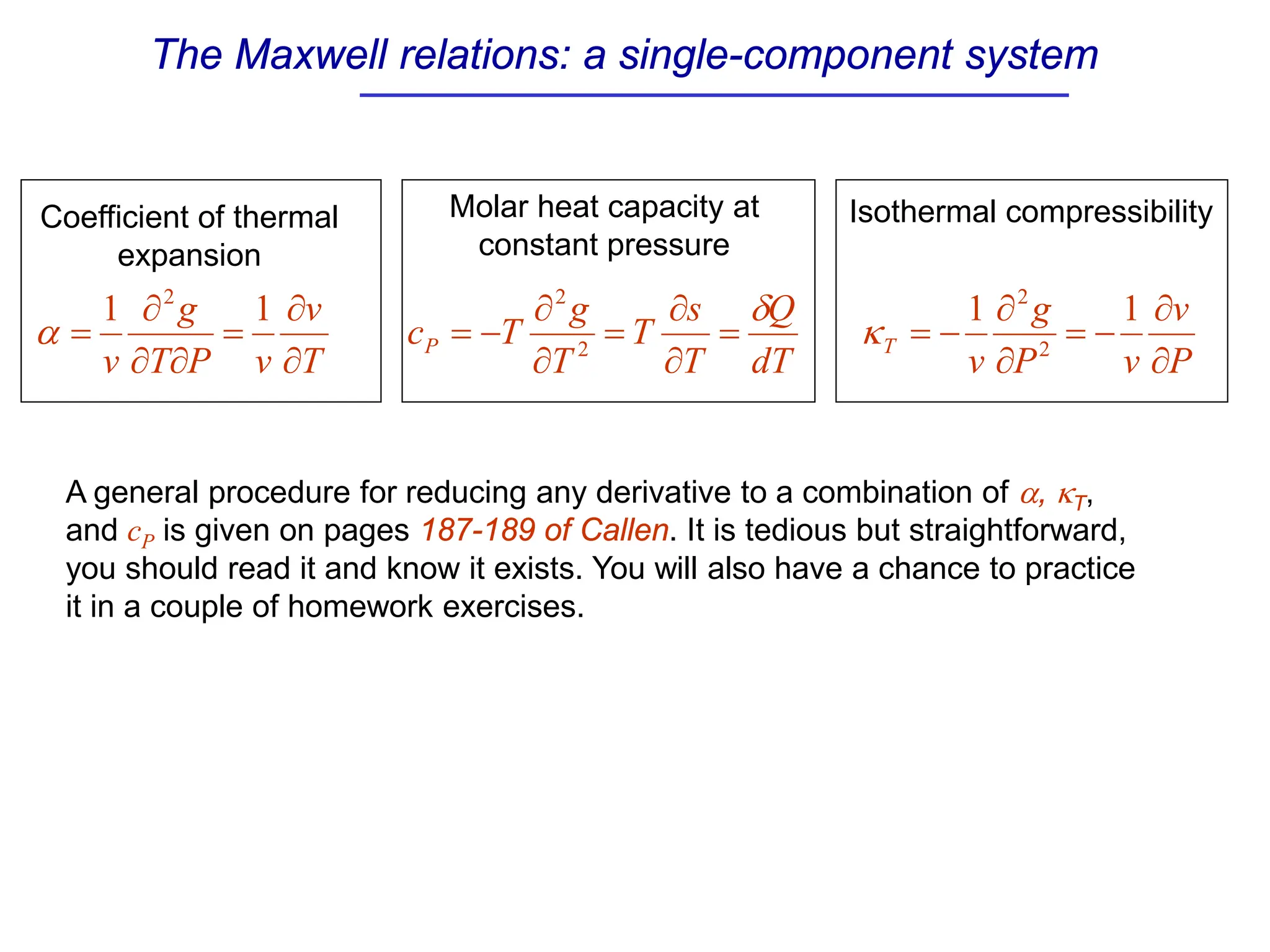
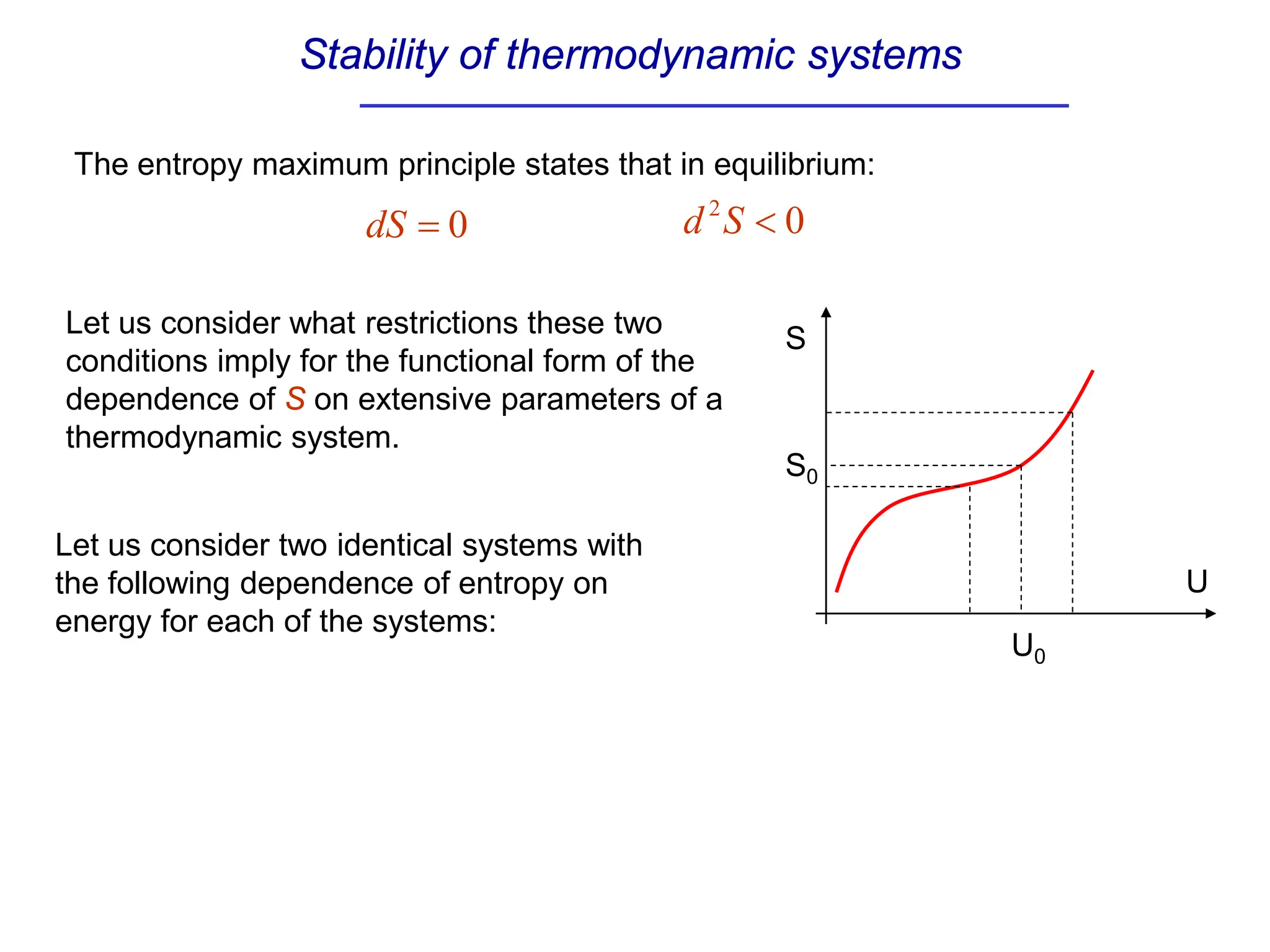
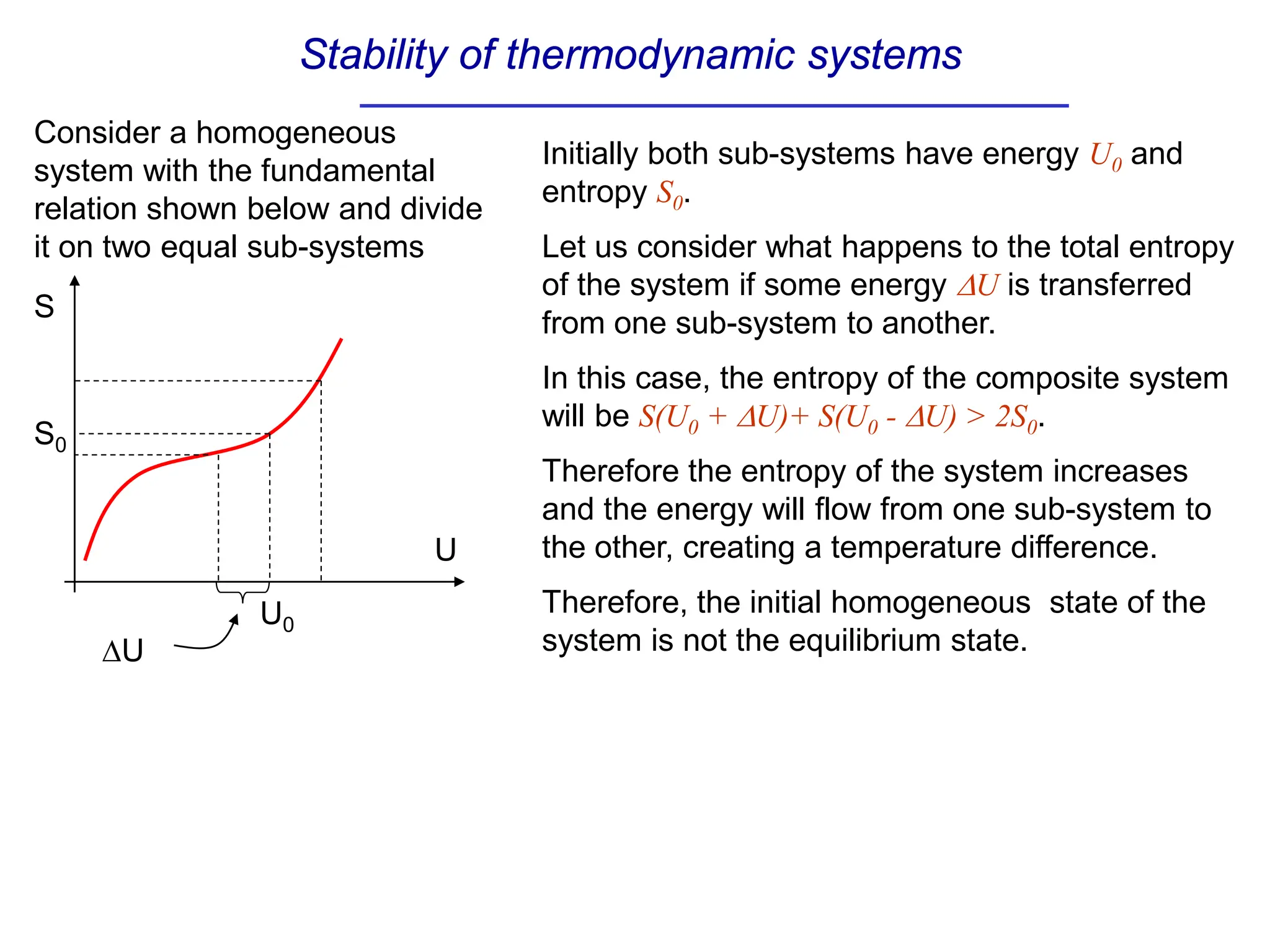
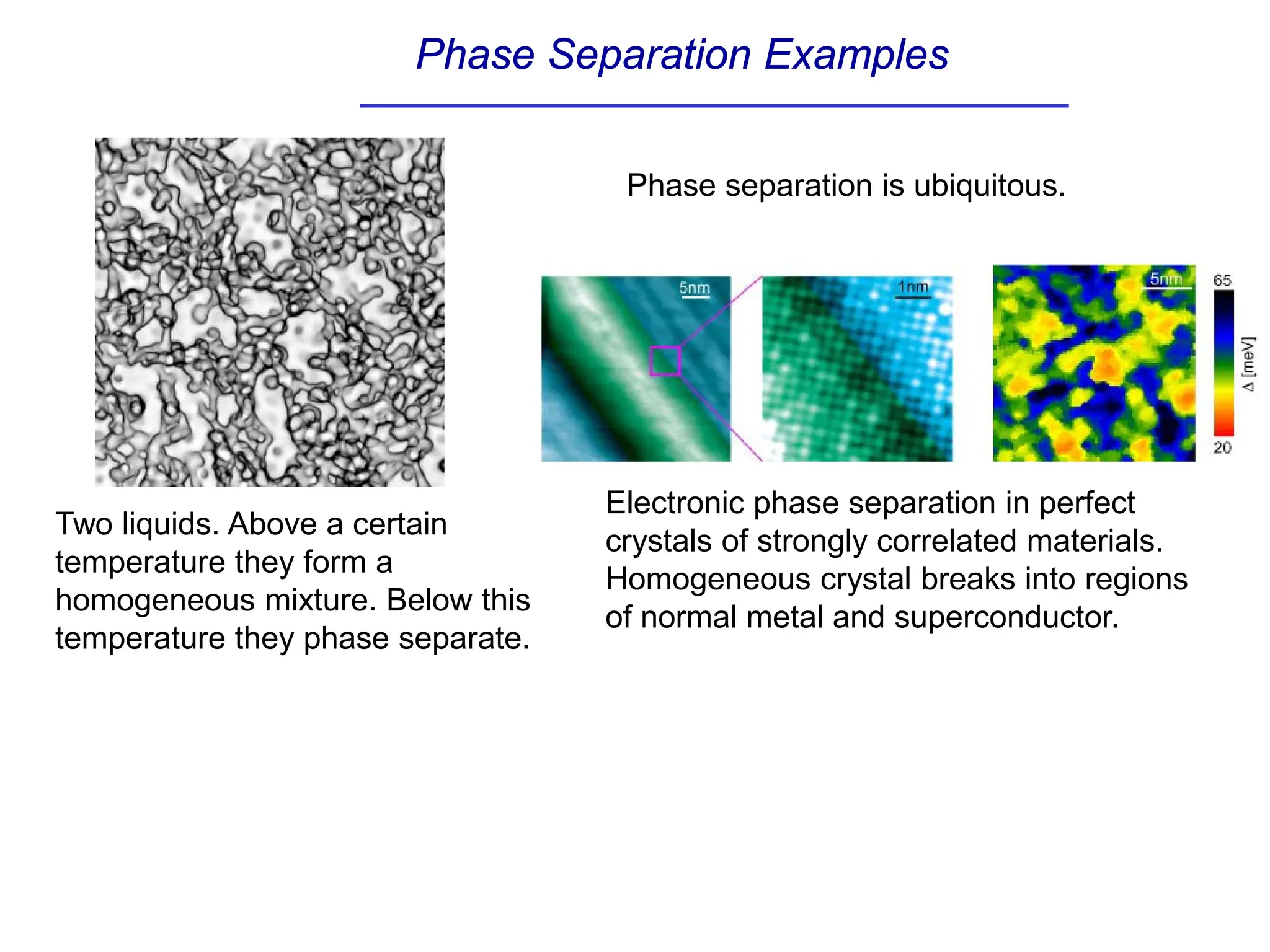
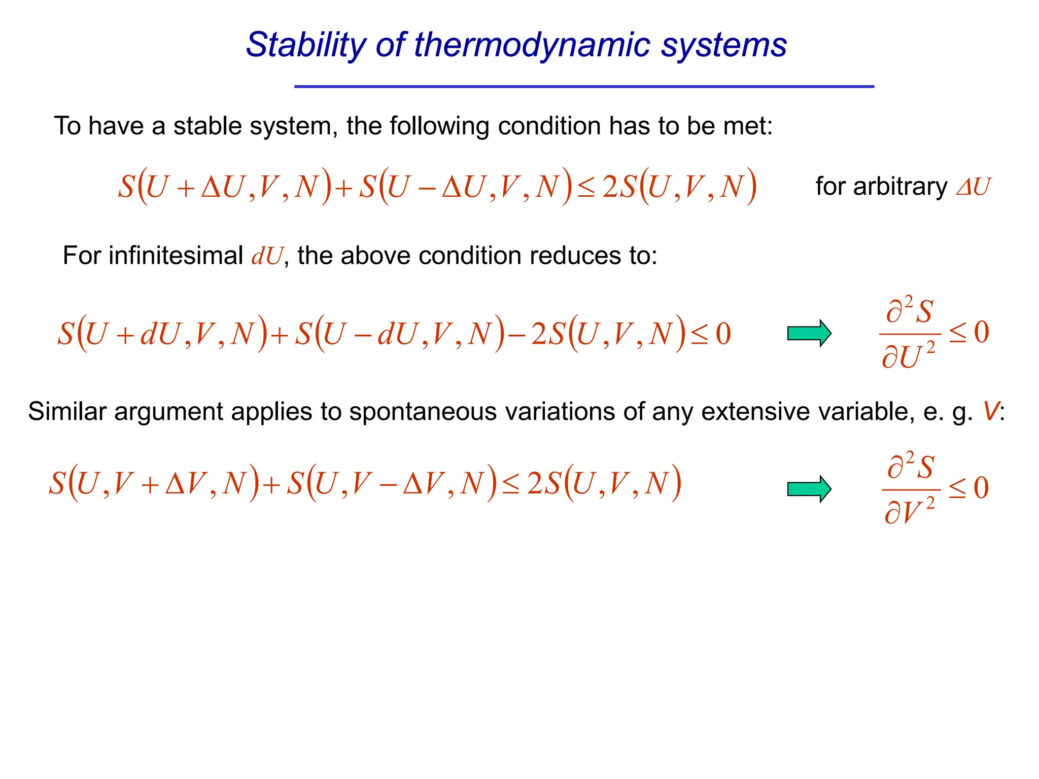
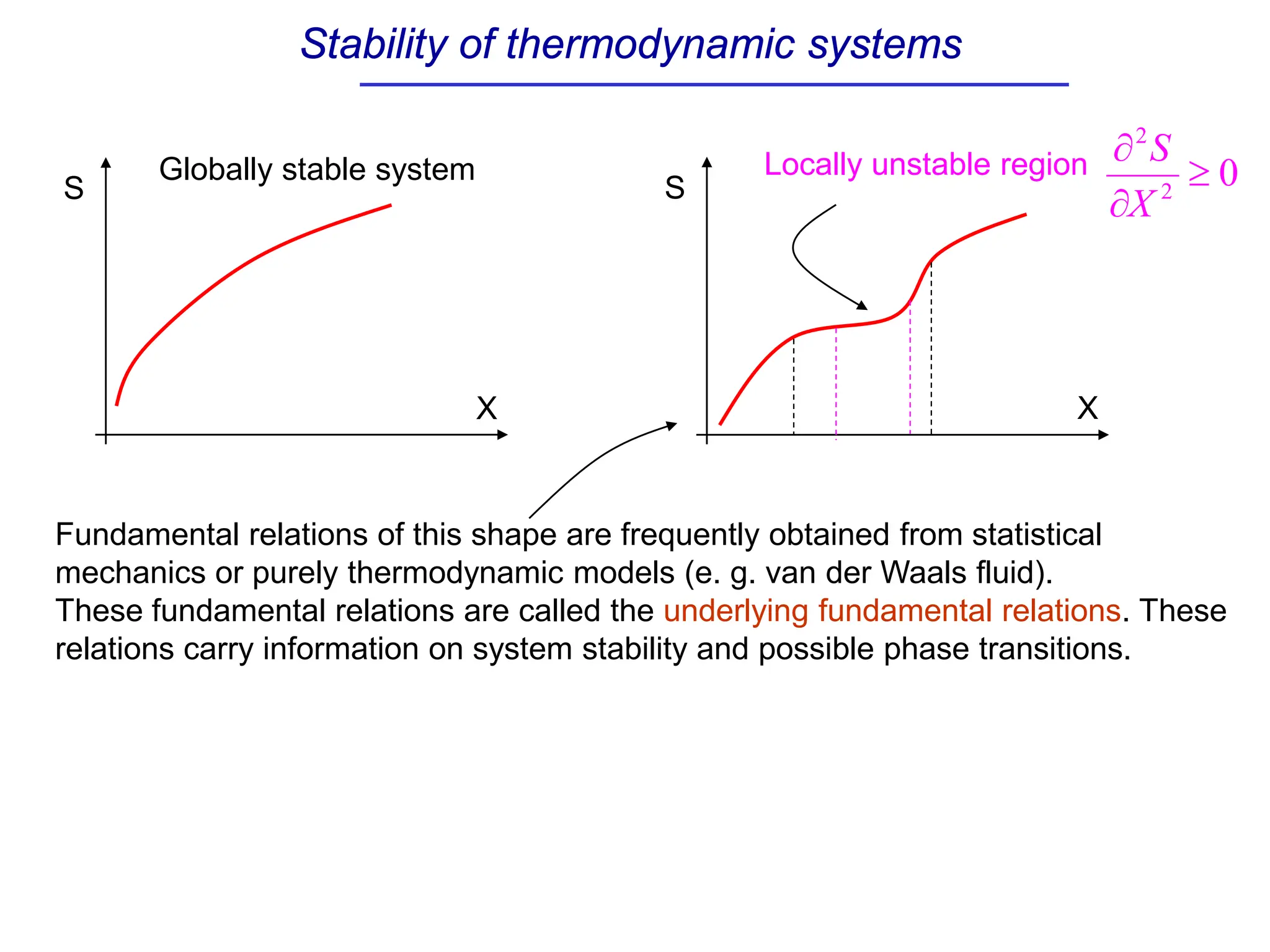
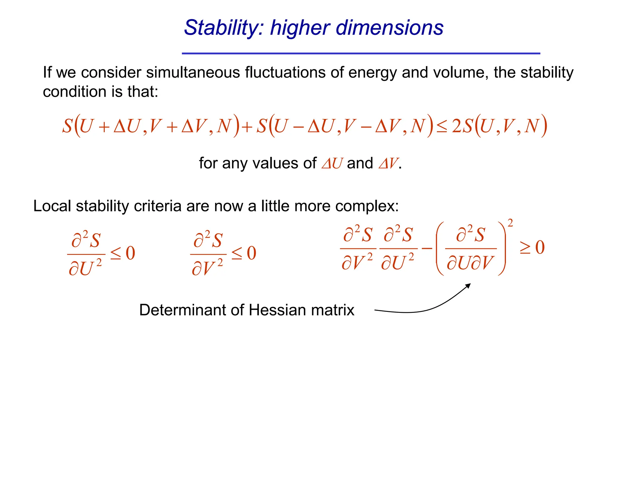
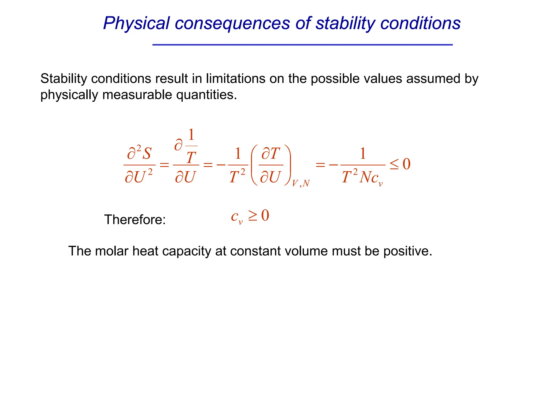
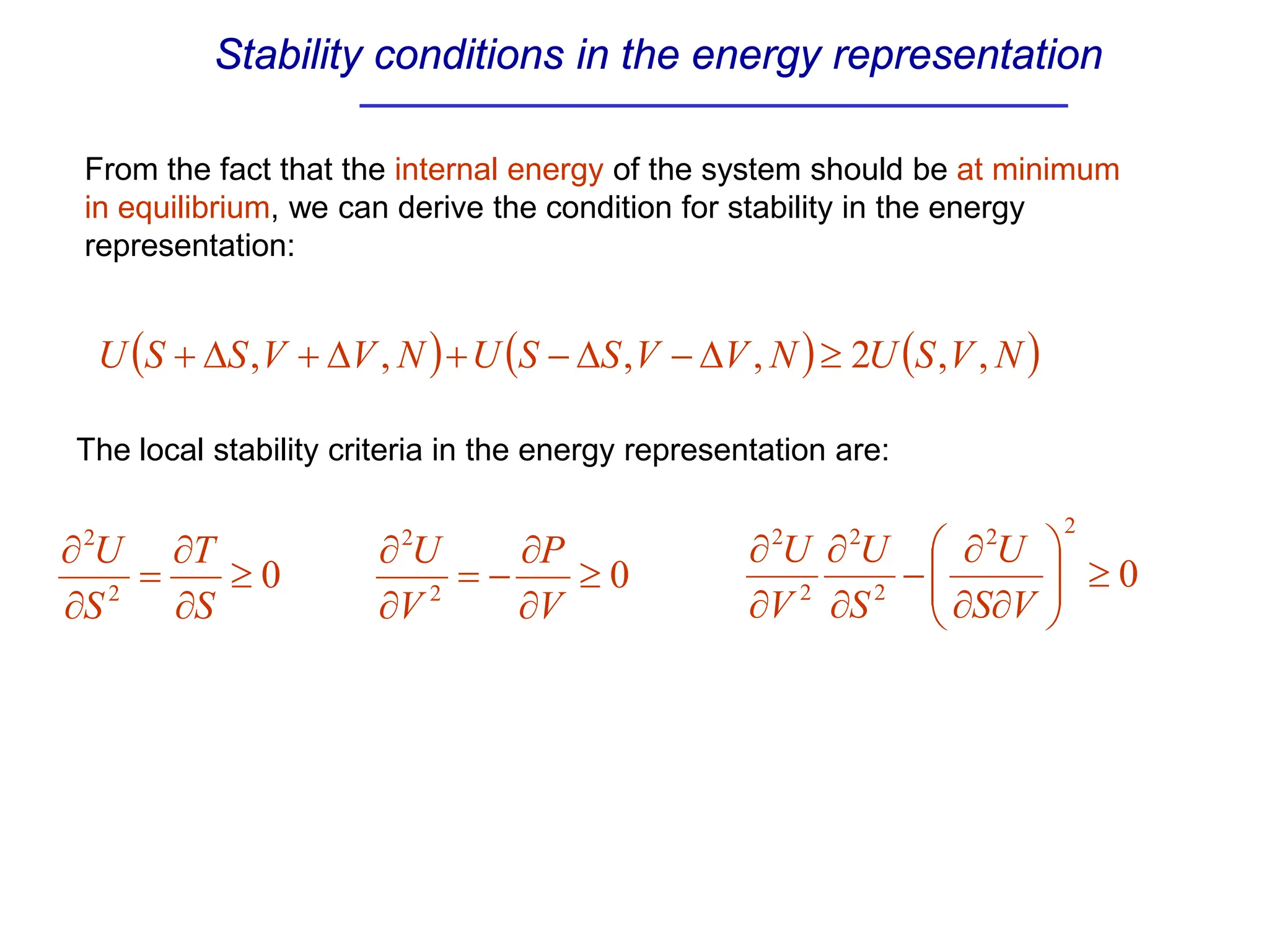
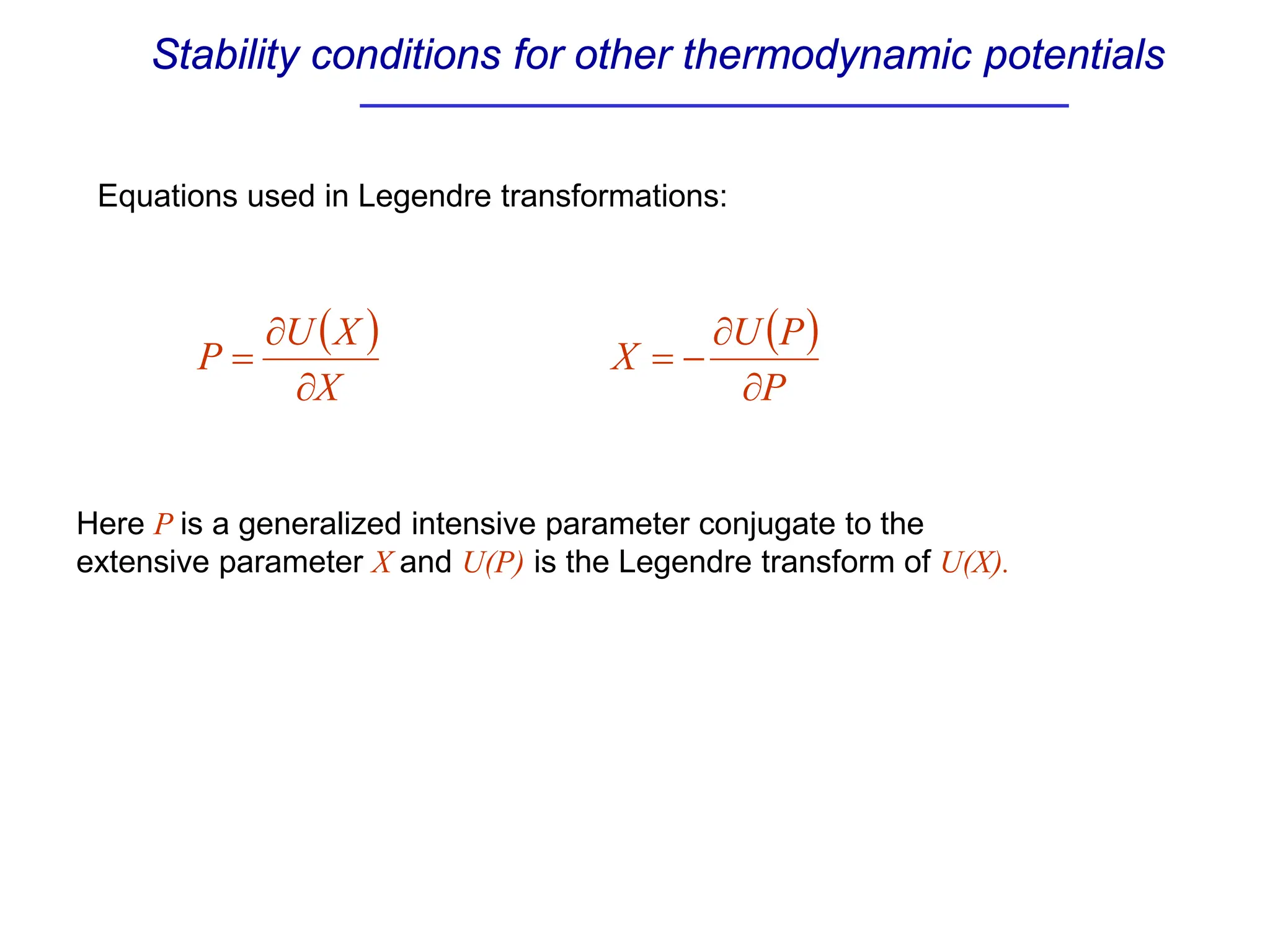
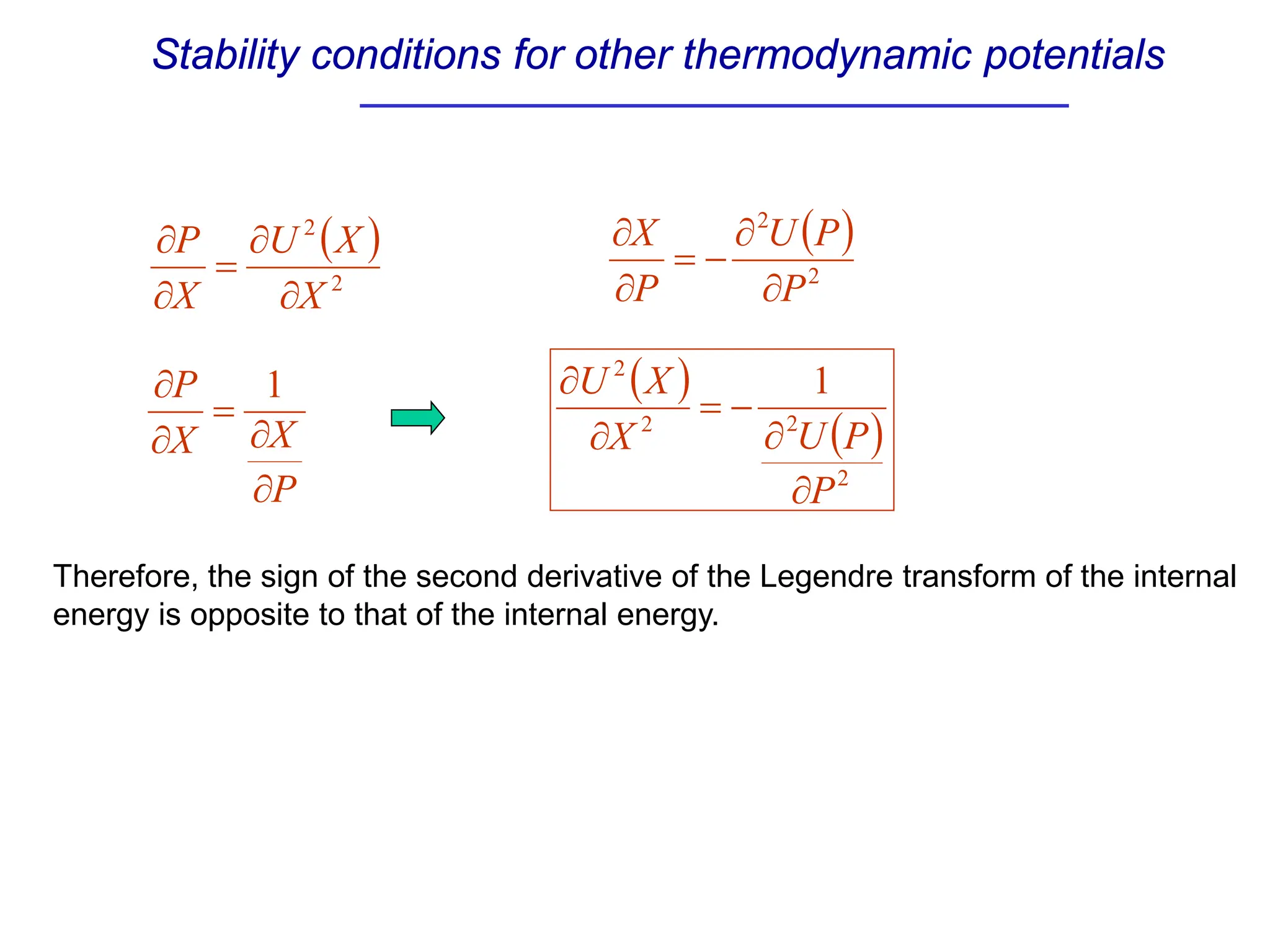
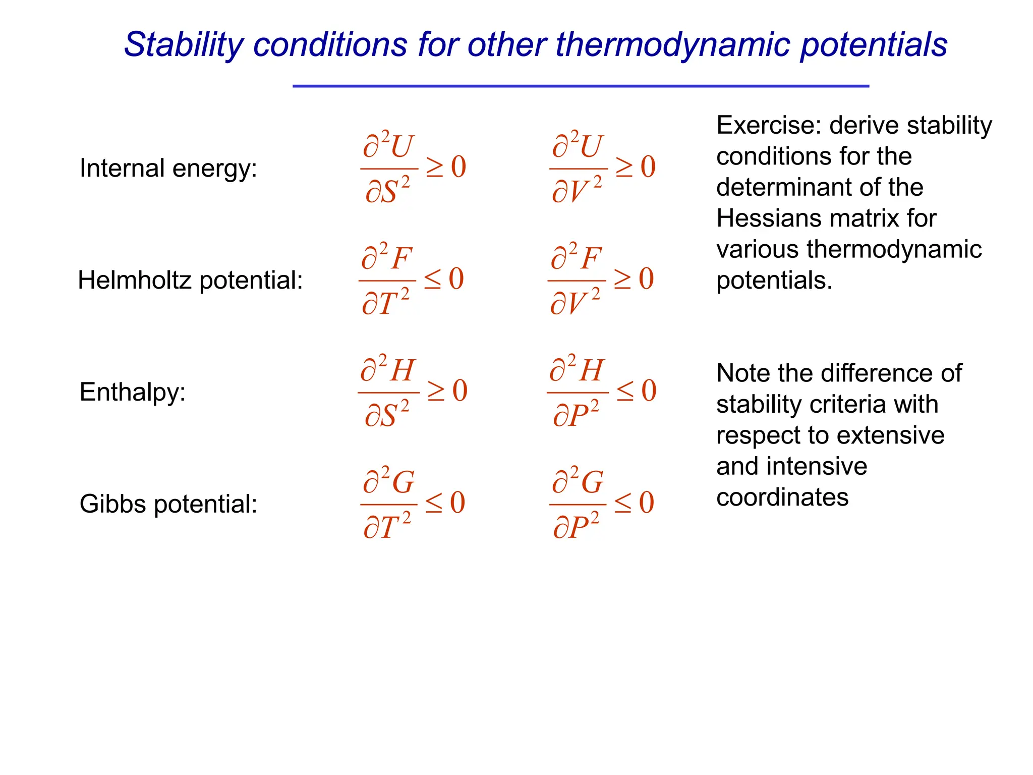
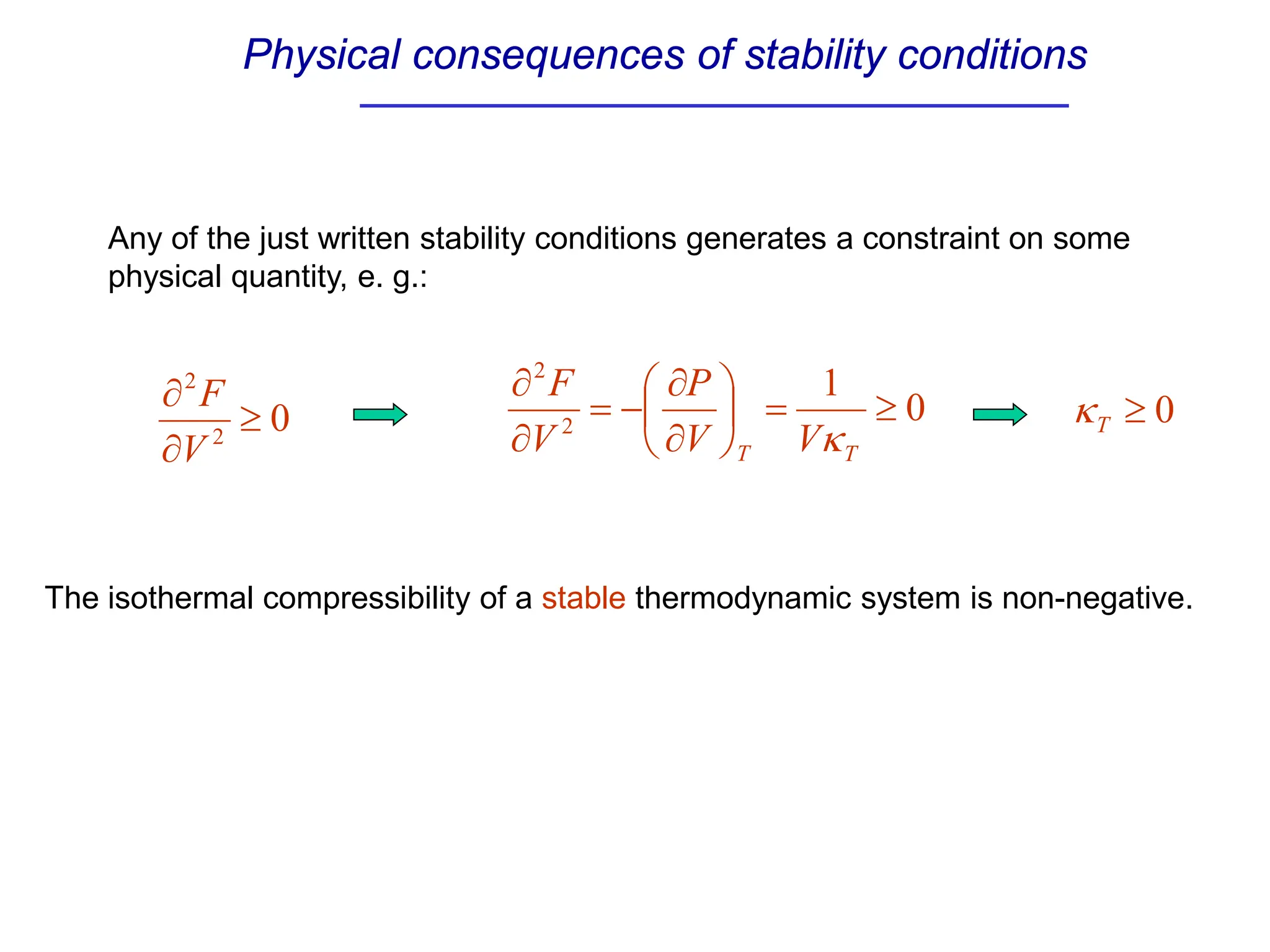
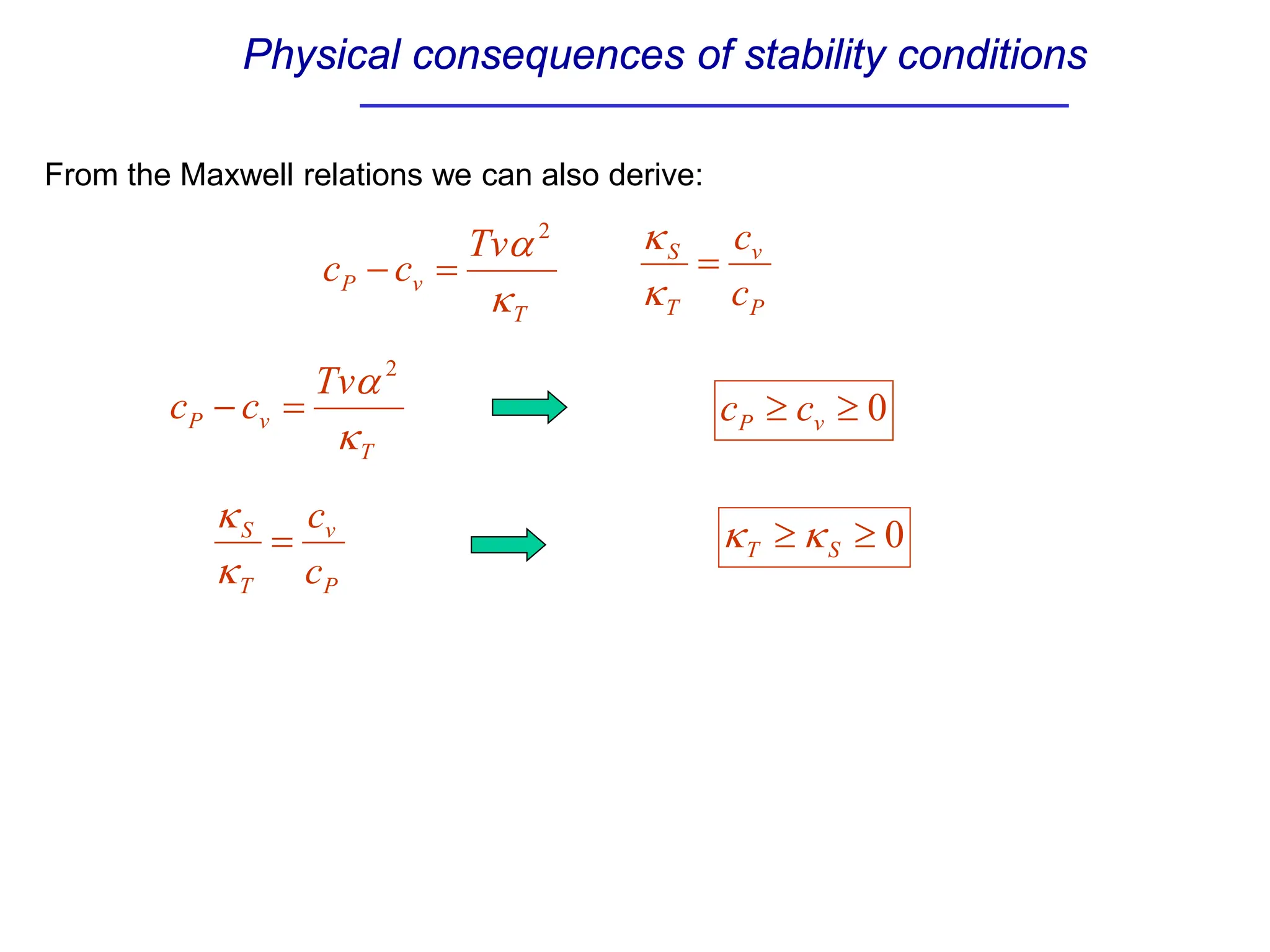
Lecture17.pdf this PPT for education and

The Maxwell relations
A number of second derivatives of the fundamental relation have clear physical
significance and can be measured experimentally. For example:
The property of the energy (or entropy) as being a differential function of its
variables gives rise to a number of relations between the second derivatives, e. g. :
S
V
U
V
S
U
∂
∂
∂
=
∂
∂
∂ 2
2
P
V
V
P
G
V
T
∂
∂
−
=
∂
∂
−
=
1
1
2
2
κ
Isothermal compressibility

S
V
U
V
S
U
∂
∂
∂
=
∂
∂
∂ 2
2
is equivalent to:
,...
,
,
,...
,
, 2
1
2
1 N
N
S
N
N
V V
T
S
P






∂
∂
=






∂
∂
−
Since this relation is not intuitively obvious, it may be regarded as a success of
thermodynamics.

Given the fact that we can write down the fundamental relation employing
various thermodynamic potentials such as F, H, G, … the number of second
derivative is large. However, the Maxwell relations reduce the number of
independent second derivatives.
Our goal is to learn how to obtain the relations among the second derivatives
without memorizing a lot of information.


















∂
∂
∂
∂
∂
∂
∂
∂
∂
∂
∂
∂
∂
∂
∂
∂
∂
∂
∂
∂
∂
∂
∂
∂
2
2
2
2
2
2
2
2
2
2
2
2
S
N
U
V
N
U
S
N
U
N
V
U
V
U
S
V
U
N
S
U
V
S
U
U
For a simple one-component system described
by the fundamental relation U(S,V,N), there are
nine second derivatives, only six of them are
independent from each other.
In general, if a thermodynamic system has n
independent coordinates, there are n(n+1)/2
independent second derivatives.

The Maxwell relations: a single-component system
For a single-component system with conserved mole number, N, there are
only three independent second derivatives:


















∂
∂
∂
∂
∂
∂
∂
∂
∂
∂
∂
∂
∂
∂
∂
∂
∂
∂
∂
∂
∂
∂
∂
∂
2
2
2
2
2
2
2
2
2
2
2
2
T
N
G
P
N
G
T
N
G
N
P
G
P
G
T
P
G
N
T
G
P
T
G
G
P
T
G
∂
∂
∂2
2
2
T
G
∂
∂
2
2
P
G
∂
∂
Other second derivatives, such as e. g.:
V
S
U
∂
∂
∂2
can all be expressed via the above three, which are trivially related to three
measurable physical parameters (dg = -sdT + vdP + µdN):

The Maxwell relations: a single-component system
A general procedure for reducing any derivative to a combination of α, κT,
and cP is given on pages 187-189 of Callen. It is tedious but straightforward,
you should read it and know it exists. You will also have a chance to practice
it in a couple of homework exercises.
T
v
v
P
T
g
v ∂
∂
=
∂
∂
∂
=
1
1 2
α
dT
Q
T
s
T
T
g
T
cP
δ
=
∂
∂
=
∂
∂
−
= 2
2
P
v
v
P
g
v
T
∂
∂
−
=
∂
∂
−
=
1
1
2
2
κ
Coefficient of thermal
expansion
Molar heat capacity at
constant pressure
Isothermal compressibility

Stability of thermodynamic systems
The entropy maximum principle states that in equilibrium:
0
=
dS 0
2
<
S
d
Let us consider what restrictions these two
conditions imply for the functional form of the
dependence of S on extensive parameters of a
thermodynamic system.
Let us consider two identical systems with
the following dependence of entropy on
energy for each of the systems:
U
S
S0
U0

Initially both sub-systems have energy U0 and
entropy S0.
Let us consider what happens to the total entropy
of the system if some energy ∆U is transferred
from one sub-system to another.
In this case, the entropy of the composite system
will be S(U0 + ∆U)+ S(U0 - ∆U) > 2S0.
Therefore the entropy of the system increases
and the energy will flow from one sub-system to
the other, creating a temperature difference.
Therefore, the initial homogeneous state of the
system is not the equilibrium state.
U
S
S0
U0
∆U
Consider a homogeneous
system with the fundamental
relation shown below and divide
it on two equal sub-systems

Phase Separation
If the homogeneous state of the system is not the equilibrium state, the
system will spontaneously become inhomogeneous, or will separate into
phases. Phases are different states of a system that have different
macroscopic parameters (e. g. density).
Phase separation takes place in phase transitions. When a system
undergoes a transition from one macroscopically different state to another it
goes through a region of phase separation (e. g. water-to-vapor phase
transition).

Phase Separation Examples
Two liquids. Above a certain
temperature they form a
homogeneous mixture. Below this
temperature they phase separate.
Electronic phase separation in perfect
crystals of strongly correlated materials.
Homogeneous crystal breaks into regions
of normal metal and superconductor.
Phase separation is ubiquitous.

To have a stable system, the following condition has to be met:
( ) ( ) ( )
N
V
U
S
N
V
U
U
S
N
V
U
U
S ,
,
2
,
,
,
, ≤
∆
−
+
∆
+ for arbitrary ∆U
For infinitesimal dU, the above condition reduces to:
( ) ( ) ( ) 0
,
,
2
,
,
,
, ≤
−
−
+
+ N
V
U
S
N
V
dU
U
S
N
V
dU
U
S 0
2
2
≤
∂
∂
U
S
Similar argument applies to spontaneous variations of any extensive variable, e. g. V:
( ) ( ) ( )
N
V
U
S
N
V
V
U
S
N
V
V
U
S ,
,
2
,
,
,
, ≤
∆
−
+
∆
+ 0
2
2
≤
∂
∂
V
S

X
S
Globally stable system
X
S
Locally unstable region
Fundamental relations of this shape are frequently obtained from statistical
mechanics or purely thermodynamic models (e. g. van der Waals fluid).
These fundamental relations are called the underlying fundamental relations. These
relations carry information on system stability and possible phase transitions.
0
2
2
≥
∂
∂
X
S

Stability: higher dimensions
( ) ( ) ( )
N
V
U
S
N
V
V
U
U
S
N
V
V
U
U
S ,
,
2
,
,
,
, ≤
∆
−
∆
−
+
∆
+
∆
+
If we consider simultaneous fluctuations of energy and volume, the stability
condition is that:
for any values of ∆U and ∆V.
0
2
2
≤
∂
∂
U
S
0
2
2
≤
∂
∂
V
S 0
2
2
2
2
2
2
≥








∂
∂
∂
−
∂
∂
∂
∂
V
U
S
U
S
V
S
Local stability criteria are now a little more complex:
Determinant of Hessian matrix

Physical consequences of stability conditions
Stability conditions result in limitations on the possible values assumed by
physically measurable quantities.
0
1
1
1
2
,
2
2
2
≤
−
=






∂
∂
−
=
∂
∂
=
∂
∂
v
N
V Nc
T
U
T
T
U
T
U
S
Therefore: 0
≥
v
c
The molar heat capacity at constant volume must be positive.

Stability conditions in the energy representation
( ) ( ) ( )
N
V
S
U
N
V
V
S
S
U
N
V
V
S
S
U ,
,
2
,
,
,
, ≥
∆
−
∆
−
+
∆
+
∆
+
From the fact that the internal energy of the system should be at minimum
in equilibrium, we can derive the condition for stability in the energy
representation:
The local stability criteria in the energy representation are:
0
2
2
≥
∂
∂
=
∂
∂
S
T
S
U
0
2
2
≥
∂
∂
−
=
∂
∂
V
P
V
U
0
2
2
2
2
2
2
≥








∂
∂
∂
−
∂
∂
∂
∂
V
S
U
S
U
V
U

Stability conditions for other thermodynamic potentials
Equations used in Legendre transformations:
( )
X
X
U
P
∂
∂
=
Here P is a generalized intensive parameter conjugate to the
extensive parameter X and U(P) is the Legendre transform of U(X).
( )
P
P
U
X
∂
∂
−
=

( )
2
2
P
P
U
P
X
∂
∂
−
=
∂
∂
( )
2
2
X
X
U
X
P
∂
∂
=
∂
∂
P
X
X
P
∂
∂
=
∂
∂ 1 ( )
( )
2
2
2
2
1
P
P
U
X
X
U
∂
∂
−
=
∂
∂
Therefore, the sign of the second derivative of the Legendre transform of the internal
energy is opposite to that of the internal energy.

0
2
2
≤
∂
∂
T
F
0
2
2
≥
∂
∂
V
F
Helmholtz potential:
0
2
2
≥
∂
∂
S
H
0
2
2
≤
∂
∂
P
H
Enthalpy:
0
2
2
≤
∂
∂
T
G
0
2
2
≤
∂
∂
P
G
Gibbs potential:
0
2
2
≥
∂
∂
S
U
0
2
2
≥
∂
∂
V
U
Internal energy:
Exercise: derive stability
conditions for the
determinant of the
Hessians matrix for
various thermodynamic
potentials.
Note the difference of
stability criteria with
respect to extensive
and intensive
coordinates

0
2
2
≥
∂
∂
V
F 0
1
2
2
≥
=






∂
∂
−
=
∂
∂
T
T V
V
P
V
F
κ
Any of the just written stability conditions generates a constraint on some
physical quantity, e. g.:
0
≥
T
κ
The isothermal compressibility of a stable thermodynamic system is non-negative.

From the Maxwell relations we can also derive:
T
v
P
Tv
c
c
κ
α 2
=
− 0
≥
≥ v
P c
c
P
v
T
S
c
c
=
κ
κ 0
≥
≥ S
T κ
κ
T
v
P
Tv
c
c
κ
α 2
=
−
P
v
T
S
c
c
=
κ
κ

Lecture17.pdf this PPT for education and

Recommended

Recommended

More Related Content

Similar to Lecture17.pdf this PPT for education and

Similar to Lecture17.pdf this PPT for education and (20)

Recently uploaded

Recently uploaded (20)

Lecture17.pdf this PPT for education and