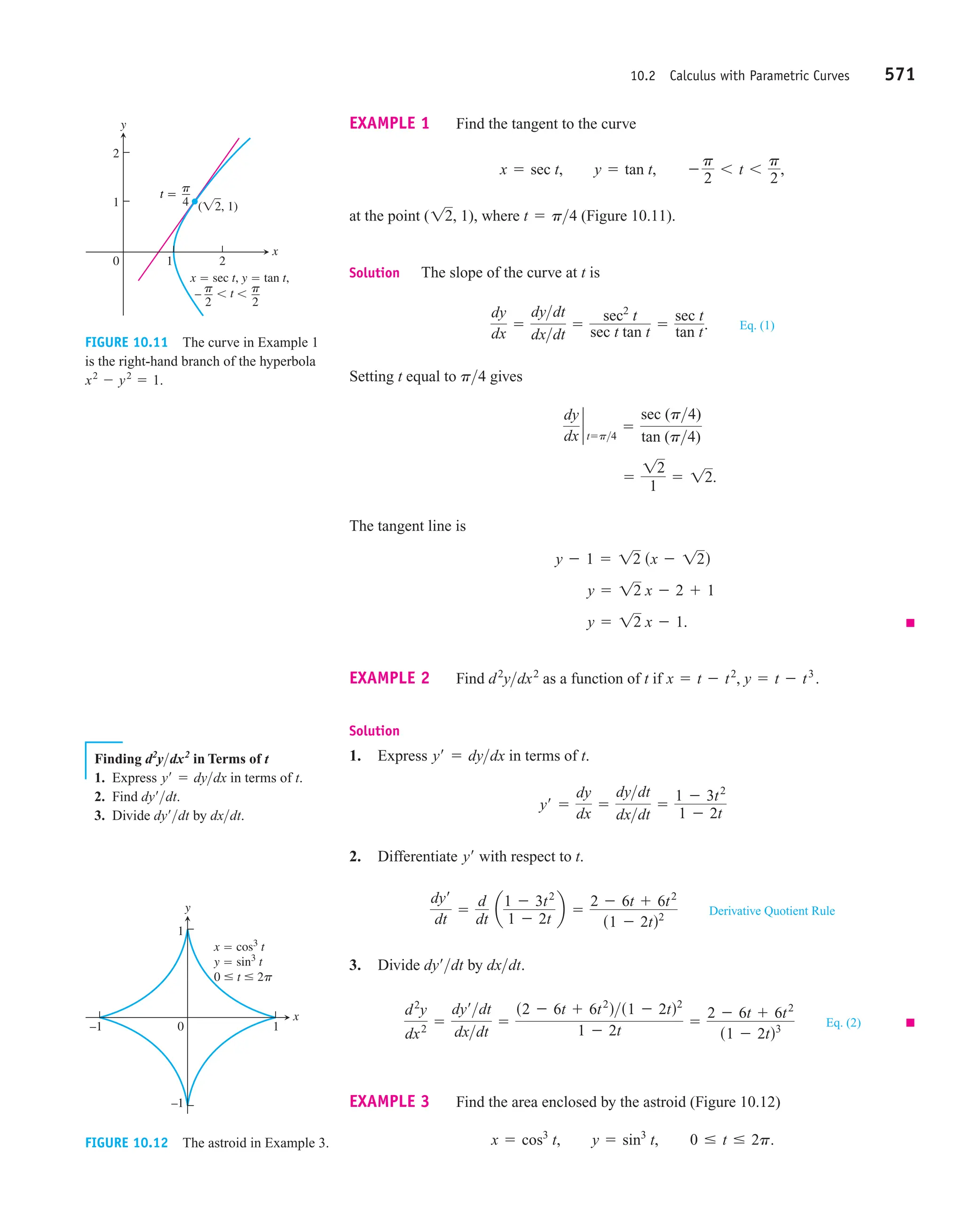
Master the language of change with the Complete Guidance Book of Calculus—your comprehensive resource for understanding the core concepts and applications of differential and integral calculus. Designed for high school, college, and self-study learners, this book takes a clear, intuitive approach to a subject often considered challenging.


![Often a function is given by a formula that describes how to calculate the output value
from the input variable. For instance, the equation is a rule that calculates the
area A of a circle from its radius r (so r, interpreted as a length, can only be positive in this
formula). When we define a function with a formula and the domain is not
stated explicitly or restricted by context, the domain is assumed to be the largest set of real
x-values for which the formula gives real y-values, the so-called natural domain. If we
want to restrict the domain in some way, we must say so. The domain of is the en-
tire set of real numbers. To restrict the domain of the function to, say, positive values of x,
we would write
Changing the domain to which we apply a formula usually changes the range as well.
The range of is The range of is the set of all numbers ob-
tained by squaring numbers greater than or equal to 2. In set notation (see Appendix 1), the
range is or or
When the range of a function is a set of real numbers, the function is said to be real-
valued. The domains and ranges of many real-valued functions of a real variable are inter-
vals or combinations of intervals. The intervals may be open, closed, or half open, and may
be finite or infinite. The range of a function is not always easy to find.
A function ƒ is like a machine that produces an output value ƒ(x) in its range whenever
we feed it an input value x from its domain (Figure 1.1).The function keys on a calculator give
an example of a function as a machine. For instance, the key on a calculator gives an out-
put value (the square root) whenever you enter a nonnegative number x and press the key.
A function can also be pictured as an arrow diagram (Figure 1.2). Each arrow associ-
ates an element of the domain D with a unique or single element in the set Y. In Figure 1.2, the
arrows indicate that ƒ(a) is associated with a, ƒ(x) is associated with x, and so on. Notice that
a function can have the same value at two different input elements in the domain (as occurs
with ƒ(a) in Figure 1.2), but each input element x is assigned a single output value ƒ(x).
EXAMPLE 1 Let’s verify the natural domains and associated ranges of some simple
functions. The domains in each case are the values of x for which the formula makes sense.
Function Domain (x) Range ( y)
[0, 1]
Solution The formula gives a real y-value for any real number x, so the domain
is The range of is because the square of any real number is
nonnegative and every nonnegative number y is the square of its own square root,
for
The formula gives a real y-value for every x except For consistency
in the rules of arithmetic, we cannot divide any number by zero. The range of the
set of reciprocals of all nonzero real numbers, is the set of all nonzero real numbers, since
That is, for the number is the input assigned to the output
value y.
The formula gives a real y-value only if The range of is
because every nonnegative number is some number’s square root (namely, it is the
square root of its own square).
In the quantity cannot be negative. That is, or
The formula gives real y-values for all The range of is the
set of all nonnegative numbers.
[0, qd,
14 - x
x … 4.
x … 4.
4 - x Ú 0,
4 - x
y = 14 - x,
[0, qd
y = 1x
x Ú 0.
y = 1x
x = 1y
y Z 0
y = 1(1y).
y = 1x,
x = 0.
y = 1x
y Ú 0.
y = A 2yB2
[0, qd
y = x2
s- q, qd.
y = x2
[-1, 1]
y = 21 - x2
[0, qd
s- q, 4]
y = 24 - x
[0, qd
[0, qd
y = 2x
s- q, 0d ´ s0, q d
s - q, 0d ´ s0, qd
y = 1x
[0, qd
s - q, qd
y = x2
2x
2x
[4, qd.
5y ƒ y Ú 46
5x2
ƒ x Ú 26
y = x2
, x Ú 2,
[0, qd.
y = x2
“y = x2
, x 7 0.”
y = x2
y = ƒsxd
A = pr2
2 Chapter 1: Functions
Input
(domain)
Output
(range)
x f(x)
f
FIGURE 1.1 A diagram showing a
function as a kind of machine.
x
a f(a) f(x)
D domain set Y set containing
the range
FIGURE 1.2 A function from a set D to a
set Y assigns a unique element of Y to each
element in D.](https://image.slidesharecdn.com/calculusbook-250617105057-211abae9/75/Complete-University-of-Calculus-2nd-edition-19-2048.jpg)
![1.1 Functions and Their Graphs 3
The formula gives a real y-value for every x in the closed interval
from to 1. Outside this domain, is negative and its square root is not a real
number. The values of vary from 0 to 1 on the given domain, and the square roots
of these values do the same. The range of is [0, 1].
Graphs of Functions
If ƒ is a function with domain D, its graph consists of the points in the Cartesian plane
whose coordinates are the input-output pairs for ƒ. In set notation, the graph is
The graph of the function is the set of points with coordinates (x, y) for
which Its graph is the straight line sketched in Figure 1.3.
The graph of a function ƒ is a useful picture of its behavior. If (x, y) is a point on the
graph, then is the height of the graph above the point x. The height may be posi-
tive or negative, depending on the sign of (Figure 1.4).
ƒsxd
y = ƒsxd
y = x + 2.
ƒsxd = x + 2
5sx, ƒsxdd ƒ x H D6.
21 - x2
1 - x2
1 - x2
-1
y = 21 - x2
x
y
–2 0
2
y x 2
FIGURE 1.3 The graph of
is the set of points (x, y) for which y has
the value x + 2.
ƒsxd = x + 2
y
x
0 1 2
x
f(x)
(x, y)
f(1)
f(2)
FIGURE 1.4 If (x, y) lies on the graph of
ƒ, then the value is the height of
the graph above the point x (or below x if
ƒ(x) is negative).
y = ƒsxd
EXAMPLE 2 Graph the function over the interval
Solution Make a table of xy-pairs that satisfy the equation . Plot the points (x, y)
whose coordinates appear in the table, and draw a smooth curve (labeled with its equation)
through the plotted points (see Figure 1.5).
How do we know that the graph of doesn’t look like one of these curves?
y = x2
y = x2
[-2, 2].
y = x2
x
4
1
0 0
1 1
2 4
9
4
3
2
-1
-2
y x 2
y x2
?
x
y
y x2
?
x
y
0 1 2
–1
–2
1
2
3
4
(–2, 4)
(–1, 1) (1, 1)
(2, 4)
⎛
⎝
⎛
⎝
3
2
9
4
,
x
y
y x2
FIGURE 1.5 Graph of the function in
Example 2.](https://image.slidesharecdn.com/calculusbook-250617105057-211abae9/75/Complete-University-of-Calculus-2nd-edition-20-2048.jpg)


![The names even and odd come from powers of x. If y is an even power of x, as in
or it is an even function of x because and If y is
an odd power of x, as in or it is an odd function of x because
and
The graph of an even function is symmetric about the y-axis. Since a
point (x, y) lies on the graph if and only if the point lies on the graph (Figure 1.12a).
A reflection across the y-axis leaves the graph unchanged.
The graph of an odd function is symmetric about the origin. Since a
point (x, y) lies on the graph if and only if the point lies on the graph (Figure 1.12b).
Equivalently, a graph is symmetric about the origin if a rotation of 180° about the origin
leaves the graph unchanged. Notice that the definitions imply that both x and must be
in the domain of ƒ.
EXAMPLE 8
Even function: for all x; symmetry about y-axis.
Even function: for all x; symmetry about y-axis
(Figure 1.13a).
Odd function: for all x; symmetry about the origin.
Not odd: but The two are not
equal.
Not even: for all (Figure 1.13b).
x Z 0
s -xd + 1 Z x + 1
-ƒsxd = -x - 1.
ƒs-xd = -x + 1,
ƒsxd = x + 1
s-xd = -x
ƒsxd = x
s-xd2
+ 1 = x2
+ 1
ƒsxd = x2
+ 1
s-xd2
= x2
ƒsxd = x2
-x
s-x, -yd
ƒs-xd = -ƒsxd,
s -x, yd
ƒs-xd = ƒsxd,
s-xd3
= -x3
.
s -xd1
= -x
y = x3
,
y = x
s-xd4
= x4
.
s-xd2
= x2
y = x4
,
y = x2
Increasing and Decreasing Functions
If the graph of a function climbs or rises as you move from left to right, we say that the
function is increasing. If the graph descends or falls as you move from left to right, the
function is decreasing.
6 Chapter 1: Functions
DEFINITIONS Let ƒ be a function defined on an interval I and let and be
any two points in I.
1. If whenever then ƒ is said to be increasing on I.
2. If whenever then ƒ is said to be decreasing on I.
x1 6 x2,
ƒsx2d 6 ƒsx1d
x1 6 x2,
ƒsx2) 7 ƒsx1d
x2
x1
x
y
1
–1
–2 2 3
–2
–1
1
2
3
y x
y ⎡x⎤
FIGURE 1.11 The graph of the
least integer function
lies on or above the line
so it provides an integer ceiling
for x (Example 6).
y = x,
y = x=
DEFINITIONS A function is an
for every x in the function’s domain.
even function of x if ƒs-xd = ƒsxd,
odd function of x if ƒs-xd = -ƒsxd,
y = ƒsxd
It is important to realize that the definitions of increasing and decreasing functions
must be satisfied for every pair of points and in I with Because we use the
inequality to compare the function values, instead of it is sometimes said that ƒ is
strictly increasing or decreasing on I. The interval I may be finite (also called bounded) or
infinite (unbounded) and by definition never consists of a single point (Appendix 1).
EXAMPLE 7 The function graphed in Figure 1.9 is decreasing on and in-
creasing on [0, 1]. The function is neither increasing nor decreasing on the interval
because of the strict inequalities used to compare the function values in the definitions.
Even Functions and Odd Functions: Symmetry
The graphs of even and odd functions have characteristic symmetry properties.
[1, qd
s - q, 0]
… ,
6
x1 6 x2.
x2
x1
(a)
(b)
0
x
y
y x2
(x, y)
(–x, y)
0
x
y
y x3
(x, y)
(–x, –y)
FIGURE 1.12 (a) The graph of
(an even function) is symmetric about the
y-axis. (b) The graph of (an odd
function) is symmetric about the origin.
y = x3
y = x2](https://image.slidesharecdn.com/calculusbook-250617105057-211abae9/75/Complete-University-of-Calculus-2nd-edition-23-2048.jpg)

![(b)
The graphs of the functions and are shown in
Figure 1.16. Both functions are defined for all (you can never divide by zero). The
graph of is the hyperbola , which approaches the coordinate axes far from
the origin. The graph of also approaches the coordinate axes. The graph of the
function ƒ is symmetric about the origin; ƒ is decreasing on the intervals and
. The graph of the function g is symmetric about the y-axis; g is increasing on
and decreasing on .
s0, q)
s- q, 0)
s0, q)
s - q, 0)
y = 1x2
xy = 1
y = 1x
x Z 0
gsxd = x-2
= 1x2
ƒsxd = x-1
= 1x
a = -1 or a = -2.
8 Chapter 1: Functions
–1 0 1
–1
1
x
y y x2
–1 1
0
–1
1
x
y y x
–1 1
0
–1
1
x
y y x3
–1 0 1
–1
1
x
y y x4
–1 0 1
–1
1
x
y y x5
FIGURE 1.15 Graphs of defined for - q 6 x 6 q .
ƒsxd = xn
, n = 1, 2, 3, 4, 5,
(a)
The graphs of for 2, 3, 4, 5, are displayed in Figure 1.15. These func-
tions are defined for all real values of x. Notice that as the power n gets larger, the curves
tend to flatten toward the x-axis on the interval and to rise more steeply for
Each curve passes through the point (1, 1) and through the origin. The graphs of
functions with even powers are symmetric about the y-axis; those with odd powers are
symmetric about the origin. The even-powered functions are decreasing on the interval
and increasing on ; the odd-powered functions are increasing over the entire
real line .
s- q, q)
[0, qd
s- q, 0]
ƒ x ƒ 7 1.
s-1, 1d,
n = 1,
ƒsxd = xn
,
a = n, a positive integer.
x
y
x
y
0
1
1
0
1
1
y
1
x y
1
x2
Domain: x 0
Range: y 0
Domain: x 0
Range: y 0
(a) (b)
FIGURE 1.16 Graphs of the power functions for part (a)
and for part (b) .
a = -2
a = -1
ƒsxd = xa
(c)
The functions and are the square root and cube
root functions, respectively. The domain of the square root function is but the
cube root function is defined for all real x. Their graphs are displayed in Figure 1.17,
along with the graphs of and (Recall that and
)
Polynomials A function p is a polynomial if
where n is a nonnegative integer and the numbers are real constants
(called the coefficients of the polynomial). All polynomials have domain If the
s - q, qd.
a0, a1, a2, Á , an
psxd = anxn
+ an-1xn-1
+ Á + a1x + a0
x23
= sx13
d2
.
x32
= sx12
d3
y = x23
.
y = x32
[0, q d,
gsxd = x13
= 2
3
x
ƒsxd = x12
= 2x
a =
1
2
,
1
3
,
3
2
, and
2
3
.](https://image.slidesharecdn.com/calculusbook-250617105057-211abae9/75/Complete-University-of-Calculus-2nd-edition-25-2048.jpg)


![14 Chapter 1: Functions
1.2
Combining Functions; Shifting and Scaling Graphs
In this section we look at the main ways functions are combined or transformed to form
new functions.
Sums, Differences, Products, and Quotients
Like numbers, functions can be added, subtracted, multiplied, and divided (except where
the denominator is zero) to produce new functions. If ƒ and g are functions, then for every
x that belongs to the domains of both ƒ and g (that is, for ), we define
functions and ƒg by the formulas
Notice that the sign on the left-hand side of the first equation represents the operation of
addition of functions, whereas the on the right-hand side of the equation means addition
of the real numbers ƒ(x) and g(x).
At any point of at which we can also define the function
by the formula
Functions can also be multiplied by constants: If c is a real number, then the function
cƒ is defined for all x in the domain of ƒ by
EXAMPLE 1 The functions defined by the formulas
have domains and The points common to these do-
mains are the points
The following table summarizes the formulas and domains for the various algebraic com-
binations of the two functions. We also write for the product function ƒg.
Function Formula Domain
[0, 1]
[0, 1]
[0, 1]
[0, 1)
(0, 1]
The graph of the function is obtained from the graphs of ƒ and g by adding the
corresponding y-coordinates ƒ(x) and g(x) at each point as in Figure 1.25.
The graphs of and from Example 1 are shown in Figure 1.26.
ƒ # g
ƒ + g
x H Dsƒd ¨ Dsgd,
ƒ + g
sx = 0 excludedd
g
ƒ
sxd =
gsxd
ƒsxd
=
A
1 - x
x
gƒ
sx = 1 excludedd
ƒ
g sxd =
ƒsxd
gsxd
=
A
x
1 - x
ƒg
sƒ # gdsxd = ƒsxdgsxd = 2xs1 - xd
ƒ # g
sg - ƒdsxd = 21 - x - 2x
g - ƒ
sƒ - gdsxd = 2x - 21 - x
ƒ - g
[0, 1] = Dsƒd ¨ Dsgd
sƒ + gdsxd = 2x + 21 - x
ƒ + g
ƒ # g
[0, qd ¨ s - q, 1] = [0, 1].
Dsgd = s- q, 1].
Dsƒd = [0, qd
ƒsxd = 2x and gsxd = 21 - x
scƒdsxd = cƒsxd.
a
ƒ
gbsxd =
ƒsxd
gsxd
swhere gsxd Z 0d.
ƒg
gsxd Z 0,
Dsƒd ¨ Dsgd
+
+
sƒgdsxd = ƒsxdgsxd.
sƒ - gdsxd = ƒsxd - gsxd.
sƒ + gdsxd = ƒsxd + gsxd.
ƒ + g, ƒ - g,
x H Dsƒd ¨ Dsgd](https://image.slidesharecdn.com/calculusbook-250617105057-211abae9/75/Complete-University-of-Calculus-2nd-edition-31-2048.jpg)
![1.2 Combining Functions; Shifting and Scaling Graphs 15
y ( f g)(x)
y g(x)
y f(x) f(a)
g(a)
f(a) g(a)
a
2
0
4
6
8
y
x
FIGURE 1.25 Graphical addition of two
functions.
5
1
5
2
5
3
5
4 1
0
1
x
y
2
1
g(x) 1 x f(x) x
y f g
y f • g
FIGURE 1.26 The domain of the function is
the intersection of the domains of ƒ and g, the
interval [0, 1] on the x-axis where these domains
overlap. This interval is also the domain of the
function (Example 1).
ƒ # g
ƒ + g
Composite Functions
Composition is another method for combining functions.
DEFINITION If ƒ and g are functions, the composite function (“ƒ com-
posed with g”) is defined by
The domain of consists of the numbers x in the domain of g for which g(x)
lies in the domain of ƒ.
ƒ ⴰ g
sƒ ⴰ gdsxd = ƒsgsxdd.
ƒ ⴰ g
The definition implies that can be formed when the range of g lies in the
domain of ƒ. To find first find g(x) and second find ƒ(g(x)). Figure 1.27 pictures
as a machine diagram and Figure 1.28 shows the composite as an arrow diagram.
ƒ ⴰ g
sƒ ⴰ gdsxd,
ƒ ⴰ g
x g f f(g(x))
g(x)
x
f(g(x))
g(x)
g
f
f g
FIGURE 1.27 A composite function uses
the output g(x) of the first function g as the input
for the second function f.
ƒ ⴰ g FIGURE 1.28 Arrow diagram for If x lies in the
domain of g and g(x) lies in the domain of f, then the
functions f and g can be composed to form (ƒ ⴰ g)(x).
ƒ ⴰ g.
To evaluate the composite function (when defined), we find ƒ(x) first and then
g(ƒ(x)). The domain of is the set of numbers x in the domain of ƒ such that ƒ(x) lies
in the domain of g.
The functions and are usually quite different.
g ⴰ ƒ
ƒ ⴰ g
g ⴰ ƒ
g ⴰ ƒ](https://image.slidesharecdn.com/calculusbook-250617105057-211abae9/75/Complete-University-of-Calculus-2nd-edition-32-2048.jpg)


![20 Chapter 1: Functions
24. The accompanying figure shows the graph of shifted to
four new positions. Write an equation for each new graph.
Exercises 25–34 tell how many units and in what directions the graphs
of the given equations are to be shifted. Give an equation for the
shifted graph. Then sketch the original and shifted graphs together,
labeling each graph with its equation.
25.
26.
27.
28.
29.
30.
31.
32.
33.
34.
Graph the functions in Exercises 35–54.
35. 36.
37. 38.
39. 40.
41. 42.
43. 44.
45. 46.
47. 48.
49. 50.
51. 52.
53. 54. y =
1
sx + 1d2
y =
1
x2
+ 1
y =
1
x2
- 1
y =
1
sx - 1d2
y =
1
x + 2
y =
1
x + 2
y =
1
x - 2
y =
1
x - 2
y = sx + 2d32
+ 1
y = 2
3
x - 1 - 1
y + 4 = x23
y = 1 - x23
y = sx - 8d23
y = sx + 1d23
y = 1 - 2x
y = 1 + 2x - 1
y = ƒ 1 - x ƒ - 1
y = ƒ x - 2 ƒ
y = 29 - x
y = 2x + 4
y = 1x2
Left 2, down 1
y = 1x Up 1, right 1
y =
1
2
sx + 1d + 5 Down 5, right 1
y = 2x - 7 Up 7
y = - 2x Right 3
y = 2x Left 0.81
y = x23
Right 1, down 1
y = x3
Left 1, down 1
x2
+ y2
= 25 Up 3, left 4
x2
+ y2
= 49 Down 3, left 2
x
y
(–2, 3)
(–4, –1)
(1, 4)
(2, 0)
(b)
(c) (d)
(a)
y = -x2 55. The accompanying figure shows the graph of a function ƒ(x) with
domain [0, 2] and range [0, 1]. Find the domains and ranges of the
following functions, and sketch their graphs.
a. b.
c. d.
e. f.
g. h.
56. The accompanying figure shows the graph of a function g(t) with
domain and range Find the domains and ranges
of the following functions, and sketch their graphs.
a. b.
c. d.
e. f.
g. h.
Vertical and Horizontal Scaling
Exercises 57–66 tell by what factor and direction the graphs of the
given functions are to be stretched or compressed. Give an equation
for the stretched or compressed graph.
57.
58.
59.
60.
61.
62.
63.
64.
65.
66. y = 1 - x3
, stretched horizontally by a factor of 2
y = 1 - x3
, compressed horizontally by a factor of 3
y = 24 - x2
, compressed vertically by a factor of 3
y = 24 - x2
, stretched horizontally by a factor of 2
y = 2x + 1, stretched vertically by a factor of 3
y = 2x + 1, compressed horizontally by a factor of 4
y = 1 +
1
x2
, stretched horizontally by a factor of 3
y = 1 +
1
x2
, compressed vertically by a factor of 2
y = x2
- 1, compressed horizontally by a factor of 2
y = x2
- 1, stretched vertically by a factor of 3
-gst - 4d
gs1 - td
gst - 2d
gs-t + 2d
1 - gstd
gstd + 3
-gstd
gs-td
t
y
–3
–2 0
–4
y g(t)
[-3, 0].
[-4, 0]
-ƒsx + 1d + 1
ƒs-xd
ƒsx - 1d
ƒsx + 2d
-ƒsxd
2ƒ(x)
ƒsxd - 1
ƒsxd + 2
x
y
0 2
1 y f(x)](https://image.slidesharecdn.com/calculusbook-250617105057-211abae9/75/Complete-University-of-Calculus-2nd-edition-37-2048.jpg)


![1.4 Graphing with Calculators and Computers 29
63. A triangle has side and angles and
Find the length a of the side opposite A.
64. The approximation sin x x It is often useful to know that,
when x is measured in radians, for numerically small val-
ues of x. In Section 3.11, we will see why the approximation holds.
The approximation error is less than 1 in 5000 if
a. With your grapher in radian mode, graph and
together in a viewing window about the origin. What do you
see happening as x nears the origin?
b. With your grapher in degree mode, graph and
together about the origin again. How is the picture dif-
ferent from the one obtained with radian mode?
General Sine Curves
For
identify A, B, C, and D for the sine functions in Exercises 65–68 and
sketch their graphs.
65. 66.
67. 68.
COMPUTER EXPLORATIONS
In Exercises 69–72, you will explore graphically the general sine
function
as you change the values of the constants A, B, C, and D. Use a CAS
or computer grapher to perform the steps in the exercises.
ƒsxd = A sin a
2p
B
sx - Cdb + D
y =
L
2p
sin
2pt
L
, L 7 0
y = -
2
p sin a
p
2
tb +
1
p
y =
1
2
sinspx - pd +
1
2
y = 2 sinsx + pd - 1
ƒsxd = A sin a
2p
B
sx - Cdb + D,
y = x
y = sin x
y = x
y = sin x
ƒ x ƒ 6 0.1.
sin x L x
L
B = p3.
A = p4
c = 2 69. The period B Set the constants
a. Plot ƒ(x) for the values over the interval
Describe what happens to the graph of the
general sine function as the period increases.
b. What happens to the graph for negative values of B? Try it
with and
70. The horizontal shift C Set the constants
a. Plot ƒ(x) for the values and 2 over the interval
Describe what happens to the graph of the
general sine function as C increases through positive values.
b. What happens to the graph for negative values of C?
c. What smallest positive value should be assigned to C so the
graph exhibits no horizontal shift? Confirm your answer with
a plot.
71. The vertical shift D Set the constants
a. Plot ƒ(x) for the values and 3 over the interval
Describe what happens to the graph of the
general sine function as D increases through positive values.
b. What happens to the graph for negative values of D?
72. The amplitude A Set the constants
a. Describe what happens to the graph of the general sine func-
tion as A increases through positive values. Confirm your an-
swer by plotting ƒ(x) for the values and 9.
b. What happens to the graph for negative values of A?
A = 1, 5,
B = 6, C = D = 0.
-4p … x … 4p.
D = 0, 1,
A = 3, B = 6, C = 0.
-4p … x … 4p.
C = 0, 1,
A = 3, B = 6, D = 0.
B = -2p.
B = -3
-4p … x … 4p.
B = 1, 3, 2p, 5p
A = 3, C = D = 0.
T
1.4
Graphing with Calculators and Computers
A graphing calculator or a computer with graphing software enables us to graph very com-
plicated functions with high precision. Many of these functions could not otherwise be
easily graphed. However, care must be taken when using such devices for graphing pur-
poses, and in this section we address some of the issues involved. In Chapter 4 we will see
how calculus helps us determine that we are accurately viewing all the important features
of a function’s graph.
Graphing Windows
When using a graphing calculator or computer as a graphing tool, a portion of the graph is
displayed in a rectangular display or viewing window. Often the default window gives an in-
complete or misleading picture of the graph. We use the term square window when the units
or scales on both axes are the same. This term does not mean that the display window itself is
square (usually it is rectangular), but instead it means that the x-unit is the same as the y-unit.
When a graph is displayed in the default window, the x-unit may differ from the y-unit of
scaling in order to fit the graph in the window. The viewing window is set by specifying an
interval [a, b] for the x-values and an interval [c, d] for the y-values. The machine selects
equally spaced x-values in [a, b] and then plots the points (x, ƒ(x)). A point is plotted if and](https://image.slidesharecdn.com/calculusbook-250617105057-211abae9/75/Complete-University-of-Calculus-2nd-edition-46-2048.jpg)
![30 Chapter 1: Functions
only if x lies in the domain of the function and ƒ(x) lies within the interval [c, d]. A short line
segment is then drawn between each plotted point and its next neighboring point. We now
give illustrative examples of some common problems that may occur with this procedure.
EXAMPLE 1 Graph the function in each of the following dis-
play or viewing windows:
(a) by (b) by (c) by
Solution
(a) We select and to specify the interval of x-values
and the range of y-values for the window. The resulting graph is shown in Figure 1.48a.
It appears that the window is cutting off the bottom part of the graph and that the in-
terval of x-values is too large. Let’s try the next window.
d = 10
a = -10, b = 10, c = -10,
[-60, 60]
[-4, 10]
[-50, 10]
[-4, 4]
[-10, 10]
[-10, 10]
ƒsxd = x3
- 7x2
+ 28
10
–10
10
–10
10
–50
4
–4
(a) (b) (c)
60
–60
10
–4
FIGURE 1.48 The graph of in different viewing windows. Selecting a window that gives a clear
picture of a graph is often a trial-and-error process (Example 1).
ƒsxd = x3
- 7x2
+ 28
(b) We see some new features of the graph (Figure 1.48b), but the top is missing and we
need to view more to the right of as well. The next window should help.
(c) Figure 1.48c shows the graph in this new viewing window. Observe that we get a
more complete picture of the graph in this window, and it is a reasonable graph of a
third-degree polynomial.
EXAMPLE 2 When a graph is displayed, the x-unit may differ from the y-unit, as in the
graphs shown in Figures 1.48b and 1.48c. The result is distortion in the picture, which may
be misleading. The display window can be made square by compressing or stretching the
units on one axis to match the scale on the other, giving the true graph. Many systems have
built-in functions to make the window “square.” If yours does not, you will have to do
some calculations and set the window size manually to get a square window, or bring to
your viewing some foreknowledge of the true picture.
Figure 1.49a shows the graphs of the perpendicular lines and
together with the semicircle in a nonsquare by display
window. Notice the distortion. The lines do not appear to be perpendicular, and the semi-
circle appears to be elliptical in shape.
Figure 1.49b shows the graphs of the same functions in a square window in which the
x-units are scaled to be the same as the y-units. Notice that the scaling on the x-axis for
Figure 1.49a has been compressed in Figure 1.49b to make the window square. Figure
1.49c gives an enlarged view of Figure 1.49b with a square by [0, 4] window.
If the denominator of a rational function is zero at some x-value within the viewing
window, a calculator or graphing computer software may produce a steep near-vertical line
segment from the top to the bottom of the window. Example 3 illustrates this situation.
[-3, 3]
[-6, 8]
[-4, 4]
y = 29 - x2
,
y = -x + 322,
y = x
x = 4](https://image.slidesharecdn.com/calculusbook-250617105057-211abae9/75/Complete-University-of-Calculus-2nd-edition-47-2048.jpg)
![1.4 Graphing with Calculators and Computers 31
(a)
8
–6
4
–4
(b)
4
–4
6
–6
(c)
4
0
3
–3
FIGURE 1.49 Graphs of the perpendicular lines and and the semicircle
appear distorted (a) in a nonsquare window, but clear (b) and (c) in square windows (Example 2).
y = 29 - x2
y = -x + 322,
y = x
(a)
10
–10
10
–10
(b)
4
–4
6
–6
FIGURE 1.50 Graphs of the function . A vertical line may appear
without a careful choice of the viewing window (Example 3).
y =
1
2 - x
EXAMPLE 3 Graph the function
Solution Figure 1.50a shows the graph in the by default square
window with our computer graphing software. Notice the near-vertical line segment at
It is not truly a part of the graph and does not belong to the domain of the
function. By trial and error we can eliminate the line by changing the viewing window to
the smaller by view, revealing a better graph (Figure 1.50b).
[-4, 4]
[-6, 6]
x = 2
x = 2.
[-10, 10]
[-10, 10]
y =
1
2 - x
.
(a)
1
–1
12
–12
(b)
1
–1
6
–6
(c)
1
–1
0.1
–0.1
FIGURE 1.51 Graphs of the function in three viewing windows. Because the period is
the smaller window in (c) best displays the true aspects of this rapidly oscillating function (Example 4).
2p100 L 0.063,
y = sin 100x
Sometimes the graph of a trigonometric function oscillates very rapidly. When a calcula-
tor or computer software plots the points of the graph and connects them, many of the maxi-
mum and minimum points are actually missed. The resulting graph is then very misleading.
EXAMPLE 4 Graph the function
Solution Figure 1.51a shows the graph of ƒ in the viewing window by
We see that the graph looks very strange because the sine curve should oscillate
periodically between and 1. This behavior is not exhibited in Figure 1.51a. We might
-1
[-1, 1].
[-12, 12]
ƒsxd = sin 100x.](https://image.slidesharecdn.com/calculusbook-250617105057-211abae9/75/Complete-University-of-Calculus-2nd-edition-48-2048.jpg)
![32 Chapter 1: Functions
experiment with a smaller viewing window, say by but the graph is not
better (Figure 1.51b). The difficulty is that the period of the trigonometric function
is very small If we choose the much smaller viewing
window by we get the graph shown in Figure 1.51c. This graph reveals
the expected oscillations of a sine curve.
EXAMPLE 5 Graph the function
Solution In the viewing window by the graph appears much like the co-
sine function with some small sharp wiggles on it (Figure 1.52a). We get a better look
when we significantly reduce the window to by [0.8, 1.02], obtaining the graph
in Figure 1.52b. We now see the small but rapid oscillations of the second term,
added to the comparatively larger values of the cosine curve.
s150d sin 50x,
[-0.6, 0.6]
[-1, 1]
[-6, 6]
y = cos x +
1
50
sin 50x.
[-1, 1]
[-0.1, 0.1]
s2p100 L 0.063d.
y = sin 100x
[-1, 1],
[-6, 6]
(a)
1
–1
6
–6
(b)
1.02
0.8
0.6
–0.6
FIGURE 1.52 In (b) we see a close-up view of the function
graphed in (a). The term cos x clearly dominates the
second term, which produces the rapid oscillations along the
cosine curve. Both views are needed for a clear idea of the graph (Example 5).
1
50
sin 50x,
y = cos x +
1
50
sin 50x
(a)
2
–2
3
–3
(b)
2
–2
3
–3
FIGURE 1.53 The graph of is missing the left branch in (a). In
(b) we graph the function obtaining both branches. (See
Example 6.)
ƒsxd =
x
ƒ x ƒ
# ƒ x ƒ
13
,
y = x13
Obtaining a Complete Graph
Some graphing devices will not display the portion of a graph for when Usu-
ally that happens because of the procedure the device is using to calculate the function val-
ues. Sometimes we can obtain the complete graph by defining the formula for the function
in a different way.
EXAMPLE 6 Graph the function
Solution Some graphing devices display the graph shown in Figure 1.53a. When we
compare it with the graph of in Figure 1.17, we see that the left branch for
y = x13
= 2
3
x
y = x13
.
x 6 0.
ƒ(x)](https://image.slidesharecdn.com/calculusbook-250617105057-211abae9/75/Complete-University-of-Calculus-2nd-edition-49-2048.jpg)
![1.5 Exponential Functions 33
is missing. The reason the graphs differ is that many calculators and computer soft-
ware programs calculate as Since the logarithmic function is not defined for
negative values of x, the computing device can produce only the right branch, where
(Logarithmic and exponential functions are introduced in the next two sections.)
To obtain the full picture showing both branches, we can graph the function
This function equals except at (where ƒ is undefined, although ). The
graph of ƒ is shown in Figure 1.53b.
013
= 0
x = 0
x13
ƒsxd =
x
ƒ x ƒ
# ƒ x ƒ13
.
x 7 0.
es13dln x
.
x13
x 6 0
Exercises 1.4
Choosing a Viewing Window
In Exercises 1–4, use a graphing calculator or computer to determine
which of the given viewing windows displays the most appropriate
graph of the specified function.
1.
a. by b. by
c. by d. by
2.
a. by b. by
c. by d. by
3.
a. by b. by
c. by d. by
4.
a. by b. by
c. by [0, 10] d. by
Finding a Viewing Window
In Exercises 5–30, find an appropriate viewing window for the given
function and use it to display its graph.
5. 6.
7. 8.
9. 10.
11. 12.
13. 14.
15. 16.
17. 18. y = 1 -
1
x + 3
y =
x + 3
x + 2
y = ƒ x2
- x ƒ
y = ƒ x2
- 1 ƒ
y = x23
s5 - xd
y = 5x25
- 2x
y = x13
sx2
- 8d
y = 2x - 3x23
ƒsxd = x2
s6 - x3
d
ƒsxd = x29 - x2
ƒsxd = 4x3
- x4
ƒsxd = x5
- 5x4
+ 10
ƒsxd =
x3
3
-
x2
2
- 2x + 1
ƒsxd = x4
- 4x3
+ 15
[-10, 10]
[-10, 10]
[-3, 7]
[-1, 4]
[-2, 6]
[-2, 2]
[-2, 2]
ƒsxd = 25 + 4x - x2
[-15, 25]
[-4, 5]
[-20, 20]
[-4, 4]
[-10, 10]
[-5, 5]
[-1, 1]
[-1, 1]
ƒsxd = 5 + 12x - x3
[-100, 100]
[-20, 20]
[-10, 20]
[-5, 5]
[-10, 10]
[-3, 3]
[-5, 5]
[-1, 1]
ƒsxd = x3
- 4x2
- 4x + 16
[-25, 15]
[-5, 5]
[-10, 10]
[-10, 10]
[-5, 5]
[-2, 2]
[-1, 1]
[-1, 1]
ƒsxd = x4
- 7x2
+ 6x
19. 20.
21. 22.
23. 24.
25. 26.
27. 28.
29. 30.
31. Graph the lower half of the circle defined by the equation
32. Graph the upper branch of the hyperbola
33. Graph four periods of the function
34. Graph two periods of the function
35. Graph the function
36. Graph the function
Graphing in Dot Mode
Another way to avoid incorrect connections when using a graphing
device is through the use of a “dot mode,” which plots only the points.
If your graphing utility allows that mode, use it to plot the functions in
Exercises 37–40.
37. 38.
39. 40. y =
x3
- 1
x2
- 1
y = x:x;
y = sin
1
x
y =
1
x - 3
ƒsxd = sin3
x.
ƒsxd = sin 2x + cos 3x.
ƒsxd = 3 cot
x
2
+ 1.
ƒsxd = - tan 2x.
y2
- 16x2
= 1.
x2
+ 2x = 4 + 4y - y2
.
y = x2
+
1
50
cos 100x
y = x +
1
10
sin 30x
y =
1
10
sin a
x
10
b
y = cos a
x
50
b
y = 3 cos 60x
y = sin 250x
ƒsxd =
x2
- 3
x - 2
ƒsxd =
6x2
- 15x + 6
4x2
- 10x
ƒsxd =
8
x2
- 9
ƒsxd =
x - 1
x2
- x - 6
ƒsxd =
x2
- 1
x2
+ 1
ƒsxd =
x2
+ 2
x2
+ 1
T
T
T
1.5
Exponential Functions
Exponential functions are among the most important in mathematics and occur in a wide
variety of applications, including interest rates, radioactive decay, population growth, the
spread of a disease, consumption of natural resources, the earth’s atmospheric pressure,
temperature change of a heated object placed in a cooler environment, and the dating of](https://image.slidesharecdn.com/calculusbook-250617105057-211abae9/75/Complete-University-of-Calculus-2nd-edition-50-2048.jpg)


![1.6 Inverse Functions and Logarithms 39
32. If John invests $2300 in a savings account with a 6% interest rate
compounded annually, how long will it take until John’s account
has a balance of $4150?
33. Doubling your money Determine how much time is required
for an investment to double in value if interest is earned at the rate
of 6.25% compounded annually.
34. Tripling your money Determine how much time is required for
an investment to triple in value if interest is earned at the rate of
5.75% compounded continuously.
35. Cholera bacteria Suppose that a colony of bacteria starts with
1 bacterium and doubles in number every half hour. How many
bacteria will the colony contain at the end of 24 hr?
36. Eliminating a disease Suppose that in any given year the num-
ber of cases of a disease is reduced by 20%. If there are 10,000
cases today, how many years will it take
a. to reduce the number of cases to 1000?
b. to eliminate the disease; that is, to reduce the number of cases
to less than 1?
1.6
Inverse Functions and Logarithms
A function that undoes, or inverts, the effect of a function ƒ is called the inverse of ƒ.
Many common functions, though not all, are paired with an inverse. In this section we
present the natural logarithmic function as the inverse of the exponential function
, and we also give examples of several inverse trigonometric functions.
One-to-One Functions
A function is a rule that assigns a value from its range to each element in its domain. Some
functions assign the same range value to more than one element in the domain. The func-
tion assigns the same value, 1, to both of the numbers and ; the sines of
and are both Other functions assume each value in their range no more
than once. The square roots and cubes of different numbers are always different. A func-
tion that has distinct values at distinct elements in its domain is called one-to-one. These
functions take on any one value in their range exactly once.
132.
2p3
p3
+1
-1
ƒsxd = x2
y = ex
y = ln x
DEFINITION A function ƒ(x) is one-to-one on a domain D if
whenever in D.
x1 Z x2
ƒsx1d Z ƒsx2d
EXAMPLE 1 Some functions are one-to-one on their entire natural domain. Other
functions are not one-to-one on their entire domain, but by restricting the function to a
smaller domain we can create a function that is one-to-one. The original and restricted
functions are not the same functions, because they have different domains. However, the
two functions have the same values on the smaller domain, so the original function is an
extension of the restricted function from its smaller domain to the larger domain.
(a) is one-to-one on any domain of nonnegative numbers because
whenever
(b) is not one-to-one on the interval because
In fact, for each element in the subinterval there is a corresponding ele-
ment in the subinterval satisfying so distinct elements in
the domain are assigned to the same value in the range. The sine function is one-to-
one on however, because it is an increasing function on giving dis-
tinct outputs for distinct inputs.
The graph of a one-to-one function can intersect a given horizontal line at
most once. If the function intersects the line more than once, it assumes the same y-value
for at least two different x-values and is therefore not one-to-one (Figure 1.57).
y = ƒsxd
[0, p2]
[0, p2],
sin x1 = sin x2,
sp2, p]
x2
[0, p2d
x1
sin sp6d = sin s5p6d.
[0, p]
gsxd = sin x
x1 Z x2.
1x2
1x1 Z
ƒsxd = 1x
0 0
(a) One-to-one: Graph meets each
horizontal line at most once.
x
y y
y x3 y x
x
FIGURE 1.57 (a) and are
one-to-one on their domains and
(b) and are not
one-to-one on their domains s- q, qd.
y = sin x
y = x2
[0, qd.
s- q, qd
y = 1x
y = x3
0
–1 1
0.5
(b) Not one-to-one: Graph meets one or
more horizontal lines more than once.
1
y
y
x x
y x2
Same y-value
Same y-value
y sin x
6
5
6](https://image.slidesharecdn.com/calculusbook-250617105057-211abae9/75/Complete-University-of-Calculus-2nd-edition-56-2048.jpg)


![increases from at to at By restricting its domain to the inter-
val we make it one-to-one, so that it has an inverse (Figure 1.63).
Similar domain restrictions can be applied to all six trigonometric functions.
sin-1
x
[-p2, p2]
x = p2.
+1
x = -p2
-1
46 Chapter 1: Functions
Domain:
Range:
x
y
1
–1
x sin y
2
2
–
y sin–1
x
–1 x 1
–/2 y /2
FIGURE 1.63 The graph of y = sin-1
x.
0
1
2
–
2
csc x
x
y
0
1
2
sec x
x
y
0
2
cot x
x
y
tan x
x
y
0
2
2
–
0
–1
1
2
cos x
x
y
x
y
0
2
2
–
sin x
–1
1
Domain:
Range: [-1, 1]
[-p2, p2]
y = sin x
Domain:
Range: [-1, 1]
[0, p]
y = cos x
Domain:
Range: s- q, qd
s-p2, p2d
y = tan x
Domain:
Range: s- q, qd
s0, pd
y = cot x
Domain:
Range: s - q, -1] ´ [1, qd
[0, p2d ´ sp2, p]
y = sec x
Domain:
Range: s- q, -1] ´ [1, qd
[-p2, 0d ´ s0, p2]
y = csc x
Domain restrictions that make the trigonometric functions one-to-one
Since these restricted functions are now one-to-one, they have inverses, which we de-
note by
These equations are read “y equals the arcsine of x” or “y equals arcsin x” and so on.
Caution The in the expressions for the inverse means “inverse.” It does not mean
reciprocal. For example, the reciprocal of sin x is
The graphs of the six inverse trigonometric functions are obtained by reflecting the
graphs of the restricted trigonometric functions through the line Figure 1.64b
shows the graph of and Figure 1.65 shows the graphs of all six functions. We
now take a closer look at two of these functions.
The Arcsine and Arccosine Functions
We define the arcsine and arccosine as functions whose values are angles (measured in ra-
dians) that belong to restricted domains of the sine and cosine functions.
y = sin-1
x
y = x.
ssin xd-1
= 1sin x = csc x.
-1
y = cot-1
x or y = arccot x
y = csc-1
x or y = arccsc x
y = sec-1
x or y = arcsec x
y = tan-1
x or y = arctan x
y = cos-1
x or y = arccos x
y = sin-1
x or y = arcsin x
x
y
x
y
1
–1
0
0 1
–1
(a)
(b)
2
2
2
–
2
–
y sin x,
2
2
– x
Domain:
Range:
[–/2, /2]
[–1, 1]
x sin y
y sin–1
x
Domain:
Range:
[–1, 1]
[–/2, /2]
FIGURE 1.64 The graphs of
(a) and
(b) its inverse, The graph of
obtained by reflection across the
line is a portion of the curve
x = sin y.
y = x,
sin-1
x,
y = sin-1
x.
y = sin x, -p2 … x … p2,](https://image.slidesharecdn.com/calculusbook-250617105057-211abae9/75/Complete-University-of-Calculus-2nd-edition-63-2048.jpg)
![1.6 Inverse Functions and Logarithms 47
The graph of (Figure 1.64b) is symmetric about the origin (it lies along the
graph of ). The arcsine is therefore an odd function:
(2)
The graph of (Figure 1.66b) has no such symmetry.
EXAMPLE 8 Evaluate (a) and (b)
Solution
(a) We see that
because and belongs to the range of the arcsine
function. See Figure 1.67a.
(b) We have
because and belongs to the range of the arccosine
function. See Figure 1.67b.
[0, p]
2p3
cos(2p3) = -12
cos-1
a-
1
2
b =
2p
3
[-p2, p2]
p3
sin(p3) = 232
sin-1
a
23
2
b =
p
3
cos-1
a-
1
2
b.
sin-1
a
23
2
b
y = cos-1
x
sin-1
s-xd = -sin-1
x.
x = sin y
y = sin-1
x
x
y
2
2
–
1
–1
(a)
Domain:
Range:
–1 x 1
y
2
–
2
y sin–1
x
x
y
2
1
–1
Domain:
Range:
–1 x 1
0 y
(b)
y cos–1
x
x
y
(c)
Domain:
Range:
–∞ x ∞
y
2
–
2
1
–1
–2 2
2
2
–
y tan–1
x
x
y
(d)
Domain:
Range:
x –1 or x 1
0 y , y
1
–1
–2 2
y sec–1
x
2
2
x
y
Domain:
Range:
x –1 or x 1
y , y 0
2
–
2
(e)
1
–1
–2 2
2
2
–
y csc–1
x
x
y
Domain:
Range: 0 y
(f)
2
1
–1
–2 2
y cot–1
x
–∞ x ∞
FIGURE 1.65 Graphs of the six basic inverse trigonometric functions.
DEFINITION
y cos1
x is the number in [0, p] for which cos y = x.
y sin1
x is the number in [-p2, p2] for which sin y = x.
The “Arc” in Arcsine
and Arccosine
For a unit circle and radian angles, the
arc length equation becomes
so central angles and the arcs they
subtend have the same measure. If
then, in addition to being the
angle whose sine is x, y is also the length
of arc on the unit circle that subtends an
angle whose sine is x. So we call y “the
arc whose sine is x.”
x = sin y,
s = u,
s = ru
Arc whose sine is x
Arc whose
cosine is x
x2
1 y2
5 1
Angle whose
sine is x
Angle whose
cosine is x
x
y
0 x 1](https://image.slidesharecdn.com/calculusbook-250617105057-211abae9/75/Complete-University-of-Calculus-2nd-edition-64-2048.jpg)
![Using the same procedure illustrated in Example 8, we can create the following table of
common values for the arcsine and arccosine functions.
48 Chapter 1: Functions
FIGURE 1.67 Values of the arcsine and arccosine functions
(Example 8).
x
y
3
0 1
2 3
3
sin
3
2
3
sin–1
3
2
(a)
0
–1
x
y
3
2
p
3
2
p
3
2
–
⎛
⎝
⎛
⎝
cos–1 1
2
p
3
2
cos –1
2
⎛
⎝
⎛
⎝
(b)
x
1 2
5p6
- 232
3p4
- 222
2p3
-12
p3
p4
222
p6
232
cos-1
x
x
1 2
-p3
- 232
-p4
- 222
-p6
-12
p6
p4
222
p3
232
sin-1
x
EXAMPLE 9 During an airplane flight from Chicago to St. Louis, the navigator deter-
mines that the plane is 12 mi off course, as shown in Figure 1.68. Find the angle a for a
course parallel to the original correct course, the angle b, and the drift correction angle
Solution From Figure 1.68 and elementary geometry, we see that and
so
Identities Involving Arcsine and Arccosine
As we can see from Figure 1.69, the arccosine of x satisfies the identity
(3)
or
(4)
Also, we can see from the triangle in Figure 1.70 that for
(5)
sin-1
x + cos-1
x = p2.
x 7 0,
cos-1
s-xd = p - cos-1
x.
cos-1
x + cos-1
s-xd = p,
c = a + b L 15°.
b = sin-1 12
62
L 0.195 radian L 11.2°
a = sin-1 12
180
L 0.067 radian L 3.8°
62 sin b = 12,
180 sin a = 12
c = a + b.
Chicago
Springfield
Plane
St. Louis
62
61 12
180
179
a
b
c
FIGURE 1.68 Diagram for drift
correction (Example 9), with distances
rounded to the nearest mile (drawing not
to scale).
FIGURE 1.69 and are
supplementary angles (so their sum is ).
p
cos-1
s-xd
cos-1
x
x
y
0
–x x
–1 1
cos–1
x
cos–1
(–x)
x
y
x
y
0
2
y cos x, 0 x
Domain:
Range:
[0, ]
[–1, 1]
y cos–1
x
Domain:
Range:
[–1, 1]
[0, ]
1
–1
(a)
(b)
2
0
–1 1
x cos y
FIGURE 1.66 The graphs of
(a) and
(b) its inverse, The graph of
obtained by reflection across the
line is a portion of the curve
x = cos y.
y = x,
cos-1
x,
y = cos-1
x.
0 … x … p,
y = cos x,](https://image.slidesharecdn.com/calculusbook-250617105057-211abae9/75/Complete-University-of-Calculus-2nd-edition-65-2048.jpg)
![1.6 Inverse Functions and Logarithms 49
Equation (5) holds for the other values of x in as well, but we cannot conclude this
from the triangle in Figure 1.70. It is, however, a consequence of Equations (2) and (4)
(Exercise 76).
The arctangent, arccotangent, arcsecant, and arccosecant functions are defined in
Section 3.9. There we develop additional properties of the inverse trigonometric functions
in a calculus setting using the identities discussed here.
[-1, 1]
1
x
cos–1
x
sin–1
x
FIGURE 1.70 and are
complementary angles (so their sum is ).
p2
cos-1
x
sin-1
x
Exercises 1.6
Identifying One-to-One Functions Graphically
Which of the functions graphed in Exercises 1–6 are one-to-one, and
which are not?
1. 2.
3. 4.
5. 6.
In Exercises 7–10, determine from its graph if the function is
one-to-one.
7.
8.
9.
10. ƒsxd = e
2 - x2
, x … 1
x2
, x 7 1
ƒsxd = d
1 -
x
2
, x … 0
x
x + 2
, x 7 0
ƒsxd = e
2x + 6, x … -3
x + 4, x 7 -3
ƒsxd = e
3 - x, x 6 0
3, x Ú 0
x
y
y x1/3
x
y
0
y
1
x
y
y int x
y
x
y 2x
x
y
0
–1 1
y x4
x2
x
y
0
y 3x3
Graphing Inverse Functions
Each of Exercises 11–16 shows the graph of a function
Copy the graph and draw in the line Then use symmetry with
respect to the line to add the graph of to your sketch. (It is
not necessary to find a formula for ) Identify the domain and
range of
11. 12.
13. 14.
15. 16.
17. a. Graph the function What
symmetry does the graph have?
b. Show that ƒ is its own inverse. (Remember that if
)
18. a. Graph the function What symmetry does the
graph have?
b. Show that ƒ is its own inverse.
ƒsxd = 1x.
x Ú 0.
2x2
= x
ƒsxd = 21 - x2
, 0 … x … 1.
x
y
0
1
–1 3
–2
x 1, 1 x 0
2 x, 0 x 3
f(x) 2
3
x
y
0
6
3
f(x) 6 2x,
0 x 3
2
2
–
y f(x) tan x,
x
x
y
0
2
2
–
x
y
0
2
2
–
1
–1
2
2
–
y f(x) sin x,
x
x
y
1
0
1
y f(x) 1 , x 0
1
x
x
y
1
0
1
y f(x) , x 0
1
x2
1
ƒ-1
.
ƒ-1
.
ƒ-1
y = x
y = x.
y = ƒsxd.](https://image.slidesharecdn.com/calculusbook-250617105057-211abae9/75/Complete-University-of-Calculus-2nd-edition-66-2048.jpg)

![1.6 Inverse Functions and Logarithms 51
In Exercises 55 and 56, solve for k.
55. a. b. c.
56. a. b. c.
In Exercises 57–60, solve for t.
57. a. b. c.
58. a. b. c.
59. 60.
Simplify the expressions in Exercises 61–64.
61. a. b. c.
d. e. f.
62. a. b. c.
d. e. f.
63. a. b. c.
64. a. b. c.
Express the ratios in Exercises 65 and 66 as ratios of natural loga-
rithms and simplify.
65. a. b. c.
66. a. b. c.
Arcsine and Arccosine
In Exercises 67–70, find the exact value of each expression.
67. a. b. c.
68. a. b. c.
69. a. b. arccos (0)
70. a. b.
Theory and Examples
71. If ƒ(x) is one-to-one, can anything be said about
Is it also one-to-one? Give reasons for your answer.
72. If ƒ(x) is one-to-one and ƒ(x) is never zero, can anything be said
about Is it also one-to-one? Give reasons for your
answer.
73. Suppose that the range of g lies in the domain of ƒ so that the
composite is defined. If ƒ and g are one-to-one, can any-
thing be said about Give reasons for your answer.
ƒ ⴰ g?
ƒ ⴰ g
hsxd = 1ƒsxd?
gsxd = -ƒsxd?
arcsin a-
1
22
b
arcsin (-1)
arccos (-1)
cos-1
a
23
2
b
cos-1
a
-1
22
b
cos-1
a
1
2
b
sin-1
a
- 23
2
b
sin-1
a
1
22
b
sin-1
a
-1
2
b
loga b
logb a
log210
x
log22 x
log9 x
log3 x
logx a
logx2 a
log2 x
log8 x
log2 x
log3 x
log4 s2ex
sin x
d
loge sex
d
25log5 s3x2
d
log2 sesln 2dssin xd
d
9log3 x
2log4 x
log3 a
1
9
b
log121 11
log11 121
plogp 7
10log10 s12d
2log2 3
log4 a
1
4
b
log323
log4 16
1.3log1.3 75
8log822
5log5 7
esx2
d
es2x+1d
= et
e2t
= x2
esln 2dt
=
1
2
ekt
=
1
10
e-0.01t
= 1000
esln 0.2dt
= 0.4
ekt
=
1
2
e-0.3t
= 27
esln 0.8dk
= 0.8
80ek
= 1
e5k
=
1
4
ek1000
= a
100e10k
= 200
e2k
= 4
74. If a composite is one-to-one, must g be one-to-one? Give
reasons for your answer.
75. Find a formula for the inverse function and verify that
a. b.
76. The identity Figure 1.70 establishes
the identity for To establish it for the rest of
verify by direct calculation that it holds for 0, and
Then, for values of x in let and apply
Eqs. (3) and (5) to the sum
77. Start with the graph of Find an equation of the graph
that results from
a. shifting down 3 units.
b. shifting right 1 unit.
c. shifting left 1, up 3 units.
d. shifting down 4, right 2 units.
e. reflecting about the y-axis.
f. reflecting about the line
78. Start with the graph of Find an equation of the graph
that results from
a. vertical stretching by a factor of 2.
b. horizontal stretching by a factor of 3.
c. vertical compression by a factor of 4.
d. horizontal compression by a factor of 2.
79. The equation has three solutions: and one
other. Estimate the third solution as accurately as you can by
graphing.
80. Could possibly be the same as for ? Graph the two
functions and explain what you see.
81. Radioactive decay The half-life of a certain radioactive sub-
stance is 12 hours. There are 8 grams present initially.
a. Express the amount of substance remaining as a function of
time t.
b. When will there be 1 gram remaining?
82. Doubling your money Determine how much time is required
for a $500 investment to double in value if interest is earned at the
rate of 4.75% compounded annually.
83. Population growth The population of Glenbrook is 375,000
and is increasing at the rate of 2.25% per year. Predict when the
population will be 1 million.
84. Radon-222 The decay equation for radon-222 gas is known to
be with t in days. About how long will it take the
radon in a sealed sample of air to fall to 90% of its original value?
y = y0e-0.18t
,
x 7 0
2ln x
xln 2
x = 2, x = 4,
x2
= 2x
y = ln x.
y = x.
y = ln x.
sin-1
s-ad + cos-1
s-ad.
x = -a, a 7 0,
s-1, 0d,
-1.
x = 1,
[-1, 1],
0 6 x 6 1.
sin-1
x + cos-1
x = P2
ƒ(x) =
50
1 + 1.1-x
ƒ(x) =
100
1 + 2-x
(ƒ-1
ⴰ ƒ)(x) = x.
(ƒ ⴰ ƒ-1
)(x) =
ƒ-1
ƒ ⴰ g
T
T](https://image.slidesharecdn.com/calculusbook-250617105057-211abae9/75/Complete-University-of-Calculus-2nd-edition-68-2048.jpg)

![2.1 Rates of Change and Tangents to Curves 53
EXAMPLE 1 A rock breaks loose from the top of a tall cliff. What is its average speed
(a) during the first 2 sec of fall?
(b) during the 1-sec interval between second 1 and second 2?
Solution The average speed of the rock during a given time interval is the change in dis-
tance, , divided by the length of the time interval, . (Increments like and are
reviewed in Appendix 3.) Measuring distance in feet and time in seconds, we have the
following calculations:
(a) For the first 2 sec:
(b) From sec 1 to sec 2:
We want a way to determine the speed of a falling object at a single instant instead of
using its average speed over an interval of time. To do this, we examine what happens
when we calculate the average speed over shorter and shorter time intervals starting at .
The next example illustrates this process. Our discussion is informal here, but it will be
made precise in Chapter 3.
EXAMPLE 2 Find the speed of the falling rock in Example 1 at and
Solution We can calculate the average speed of the rock over a time interval
having length as
(1)
We cannot use this formula to calculate the “instantaneous” speed at the exact moment
by simply substituting because we cannot divide by zero. But we can use it to cal-
culate average speeds over increasingly short time intervals starting at and
When we do so, we see a pattern (Table 2.1).
t0 = 2.
t0 = 1
h = 0,
t0
¢y
¢t
=
16st0 + hd2
- 16t0
2
h
.
¢t = h,
[t0, t0 + h],
t = 2 sec.
t = 1
t0
t0,
¢y
¢t
=
16s2d2
- 16s1d2
2 - 1
= 48
ft
sec
¢y
¢t
=
16s2d2
- 16s0d2
2 - 0
= 32
ft
sec
¢t
¢y
¢t
¢y
TABLE 2.1 Average speeds over short time intervals
Length of Average speed over Average speed over
time interval interval of length h interval of length h
h starting at starting at
1 48 80
0.1 33.6 65.6
0.01 32.16 64.16
0.001 32.016 64.016
0.0001 32.0016 64.0016
t0 2
t0 1
Average speed:
¢y
¢t
=
16st0 + hd2
- 16t0
2
h
[t0, t0 + h]
The average speed on intervals starting at seems to approach a limiting value
of 32 as the length of the interval decreases. This suggests that the rock is falling at a speed
of 32 ft sec at Let’s confirm this algebraically.
t0 = 1 sec.
t0 = 1](https://image.slidesharecdn.com/calculusbook-250617105057-211abae9/75/Complete-University-of-Calculus-2nd-edition-70-2048.jpg)
![54 Chapter 2: Limits and Continuity
If we set and then expand the numerator in Equation (1) and simplify, we find that
For values of h different from 0, the expressions on the right and left are equivalent and the
average speed is We can now see why the average speed has the limiting
value as h approaches 0.
Similarly, setting in Equation (1), the procedure yields
for values of h different from 0. As h gets closer and closer to 0, the average speed has the
limiting value 64 ft sec when as suggested by Table 2.1.
The average speed of a falling object is an example of a more general idea which we
discuss next.
Average Rates of Change and Secant Lines
Given an arbitrary function we calculate the average rate of change of y with
respect to x over the interval by dividing the change in the value of y,
by the length of the interval over which the
change occurs. (We use the symbol h for to simplify the notation here and later on.)
¢x
¢x = x2 - x1 = h
¢y = ƒsx2d - ƒsx1d,
[x1, x2]
y = ƒsxd,
t0 = 2 sec,
¢y
¢t
= 64 + 16h
t0 = 2
32 + 16s0d = 32 ftsec
32 + 16h ftsec.
=
32h + 16h2
h
= 32 + 16h.
¢y
¢t
=
16s1 + hd2
- 16s1d2
h
=
16s1 + 2h + h2
d - 16
h
t0 = 1
DEFINITION The average rate of change of with respect to x over the
interval is
¢y
¢x
=
ƒsx2d - ƒsx1d
x2 - x1
=
ƒsx1 + hd - ƒsx1d
h
, h Z 0.
[x1, x2]
y = ƒsxd
y
x
0
Secant
P(x1, f(x1))
Q(x2, f(x2))
x h
y
x2
x1
y f(x)
FIGURE 2.1 A secant to the graph
Its slope is the
average rate of change of ƒ over the
interval [x1 , x2].
¢y¢x,
y = ƒsxd.
Geometrically, the rate of change of ƒ over is the slope of the line through the points
and (Figure 2.1). In geometry, a line joining two points of a curve
is a secant to the curve. Thus, the average rate of change of ƒ from to is identical with
the slope of secant PQ. Let’s consider what happens as the point Q approaches the point P
along the curve, so the length h of the interval over which the change occurs approaches
zero. We will see that this procedure leads to defining the slope of a curve at a point.
Defining the Slope of a Curve
We know what is meant by the slope of a straight line, which tells us the rate at which it
rises or falls—its rate of change as a linear function. But what is meant by the slope of a
curve at a point P on the curve? If there is a tangent line to the curve at P—a line that just
touches the curve like the tangent to a circle—it would be reasonable to identify the slope
of the tangent as the slope of the curve at P. So we need a precise meaning for the tangent
at a point on a curve.
For circles, tangency is straightforward. A line L is tangent to a circle at a point P if L
passes through P perpendicular to the radius at P (Figure 2.2). Such a line just touches the circle.
But what does it mean to say that a line L is tangent to some other curve C at a point P?
x2
x1
Qsx2, ƒsx2dd
Psx1, ƒsx1dd
[x1, x2]
P
L
O
FIGURE 2.2 L is tangent to the
circle at P if it passes through P
perpendicular to radius OP.](https://image.slidesharecdn.com/calculusbook-250617105057-211abae9/75/Complete-University-of-Calculus-2nd-edition-71-2048.jpg)


![2.1 Rates of Change and Tangents to Curves 57
FIGURE 2.6 The positions and slopes of four secants through the point P on the fruit fly graph (Example 5).
Slope of
Q (flies day)
(45, 340)
(40, 330)
(35, 310)
(30, 265)
265 - 150
30 - 23
L 16.4
310 - 150
35 - 23
L 13.3
330 - 150
40 - 23
L 10.6
340 - 150
45 - 23
L 8.6
/
PQ ≤p/≤t
t
Number
of
flies
p
350
300
250
200
150
100
50
0 10 20 30 40 50
Time (days)
Number
of
flies
A(14, 0)
P(23, 150)
B(35, 350)
Q(45, 340)
The values in the table show that the secant slopes rise from 8.6 to 16.4 as the
t-coordinate of Q decreases from 45 to 30, and we would expect the slopes to rise slightly
higher as t continued on toward 23. Geometrically, the secants rotate about P and seem to
approach the red tangent line in the figure. Since the line appears to pass through the
points (14, 0) and (35, 350), it has slope
(approximately).
On day 23 the population was increasing at a rate of about 16.7 flies day.
The instantaneous rates in Example 2 were found to be the values of the average
speeds, or average rates of change, as the time interval of length h approached 0. That is,
the instantaneous rate is the value the average rate approaches as the length h of the in-
terval over which the change occurs approaches zero. The average rate of change corre-
sponds to the slope of a secant line; the instantaneous rate corresponds to the slope of
the tangent line as the independent variable approaches a fixed value. In Example 2, the
independent variable t approached the values and . In Example 3, the inde-
pendent variable x approached the value . So we see that instantaneous rates and
slopes of tangent lines are closely connected. We investigate this connection thoroughly
in the next chapter, but to do so we need the concept of a limit.
x = 2
t = 2
t = 1
350 - 0
35 - 14
= 16.7 fliesday
Exercises 2.1
Average Rates of Change
In Exercises 1–6, find the average rate of change of the function over
the given interval or intervals.
1.
a. [2, 3] b.
2.
a. b.
3.
a. b.
4.
a. b. [-p, p]
[0, p]
gstd = 2 + cos t
[p6, p2]
[p4, 3p4]
hstd = cot t
[-2, 0]
[-1, 1]
gsxd = x2
[-1, 1]
ƒsxd = x3
+ 1
5.
6.
Slope of a Curve at a Point
In Exercises 7–14, use the method in Example 3 to find (a) the slope
of the curve at the given point P, and (b) an equation of the tangent
line at P.
7.
8.
9.
10.
11. y = x3
, P(2, 8)
y = x2
- 4x, P(1, -3)
y = x2
- 2x - 3, P(2, -3)
y = 5 - x2
, P(1, 4)
y = x2
- 3, P(2, 1)
Psud = u3
- 4u2
+ 5u; [1, 2]
Rsud = 24u + 1; [0, 2]](https://image.slidesharecdn.com/calculusbook-250617105057-211abae9/75/Complete-University-of-Calculus-2nd-edition-74-2048.jpg)
![58 Chapter 2: Limits and Continuity
T
12.
13.
14.
Instantaneous Rates of Change
15. Speed of a car The accompanying figure shows the time-
to-distance graph for a sports car accelerating from a standstill.
a. Estimate the slopes of secants and
arranging them in order in a table like the one in Figure 2.6.
What are the appropriate units for these slopes?
b. Then estimate the car’s speed at time
16. The accompanying figure shows the plot of distance fallen versus
time for an object that fell from the lunar landing module a dis-
tance 80 m to the surface of the moon.
a. Estimate the slopes of the secants and
arranging them in a table like the one in Figure 2.6.
b. About how fast was the object going when it hit the surface?
17. The profits of a small company for each of the first five years of
its operation are given in the following table:
a. Plot points representing the profit as a function of year, and
join them by as smooth a curve as you can.
Year Profit in $1000s
2000 6
2001 27
2002 62
2003 111
2004 174
t
y
0
20
Elapsed time (sec)
Distance
fallen
(m)
5 10
P
40
60
80
Q1
Q2
Q3
Q4
PQ4 ,
PQ1 , PQ2 , PQ3 ,
t = 20 sec.
PQ4 ,
PQ1 , PQ2 , PQ3 ,
0 5
200
100
Elapsed time (sec)
Distance
(m)
10 15 20
300
400
500
600
650
P
Q1
Q2
Q3
Q4
t
s
y = x3
- 3x2
+ 4, P(2, 0)
y = x3
- 12x, P(1, -11)
y = 2 - x3
, P(1, 1) b. What is the average rate of increase of the profits between
2002 and 2004?
c. Use your graph to estimate the rate at which the profits were
changing in 2002.
18. Make a table of values for the function
at the points
and
a. Find the average rate of change of F(x) over the intervals [1, x]
for each in your table.
b. Extending the table if necessary, try to determine the rate of
change of F(x) at
19. Let for
a. Find the average rate of change of g(x) with respect to x over
the intervals [1, 2], [1, 1.5] and
b. Make a table of values of the average rate of change of g with
respect to x over the interval for some values of h
approaching zero, say
and 0.000001.
c. What does your table indicate is the rate of change of g(x)
with respect to x at
d. Calculate the limit as h approaches zero of the average rate of
change of g(x) with respect to x over the interval
20. Let for
a. Find the average rate of change of ƒ with respect to t over the
intervals (i) from to and (ii) from to
b. Make a table of values of the average rate of change of ƒ with
respect to t over the interval [2, T], for some values of T ap-
proaching 2, say and
2.000001.
c. What does your table indicate is the rate of change of ƒ with
respect to t at
d. Calculate the limit as T approaches 2 of the average rate of
change of ƒ with respect to t over the interval from 2 to T. You
will have to do some algebra before you can substitute
21. The accompanying graph shows the total distance s traveled by a
bicyclist after t hours.
a. Estimate the bicyclist’s average speed over the time intervals
[0, 1], [1, 2.5], and [2.5, 3.5].
b. Estimate the bicyclist’s instantaneous speed at the times
and .
c. Estimate the bicyclist’s maximum speed and the specific time
at which it occurs.
t = 3
t = 2,
t = 1
2,
1
0
10
20
30
40
2 3 4
Elapsed time (hr)
Distance
traveled
(mi)
t
s
T = 2.
t = 2?
T = 2.1, 2.01, 2.001, 2.0001, 2.00001,
t = T.
t = 2
t = 3,
t = 2
t Z 0.
ƒstd = 1t
[1, 1 + h].
x = 1?
h = 0.1, 0.01, 0.001, 0.0001, 0.00001,
[1, 1 + h]
[1, 1 + h].
x Ú 0.
gsxd = 2x
x = 1.
x Z 1
x = 1.
x = 1000110000,
x = 10011000,
x = 1.2, x = 1110, x = 101100,
Fsxd = sx + 2dsx - 2d
T
T
T](https://image.slidesharecdn.com/calculusbook-250617105057-211abae9/75/Complete-University-of-Calculus-2nd-edition-75-2048.jpg)
![22. The accompanying graph shows the total amount of gasoline A in
the gas tank of an automobile after being driven for t days.
3
1
0
4
8
12
16
5
2 6 7 8 9
4 10
Elapsed time (days)
Remaining
amount
(gal)
t
A
2.2 Limit of a Function and Limit Laws 59
a. Estimate the average rate of gasoline consumption over the
time intervals [0, 3], [0, 5], and [7, 10].
b. Estimate the instantaneous rate of gasoline consumption at
the times , , and .
c. Estimate the maximum rate of gasoline consumption and the
specific time at which it occurs.
t = 8
t = 4
t = 1
2.2 Limit of a Function and Limit Laws
In Section 2.1 we saw that limits arise when finding the instantaneous rate of change of a
function or the tangent to a curve. Here we begin with an informal definition of limit and
show how we can calculate the values of limits. A precise definition is presented in the
next section.
Limits of Function Values
Frequently when studying a function , we find ourselves interested in the func-
tion’s behavior near a particular point c, but not at c. This might be the case, for instance,
if c is an irrational number, like or , whose values can only be approximated by
“close” rational numbers at which we actually evaluate the function instead. Another situa-
tion occurs when trying to evaluate a function at c leads to division by zero, which is unde-
fined. We encountered this last circumstance when seeking the instantaneous rate of
change in y by considering the quotient function for h closer and closer to zero.
Here’s a specific example where we explore numerically how a function behaves near a
particular point at which we cannot directly evaluate the function.
EXAMPLE 1 How does the function
behave near
Solution The given formula defines ƒ for all real numbers x except (we cannot di-
vide by zero). For any we can simplify the formula by factoring the numerator and
canceling common factors:
The graph of ƒ is the line with the point (1, 2) removed. This removed point is
shown as a “hole” in Figure 2.7. Even though ƒ(1) is not defined, it is clear that we can
make the value of ƒ(x) as close as we want to 2 by choosing x close enough to 1 (Table 2.2).
y = x + 1
ƒsxd =
sx - 1dsx + 1d
x - 1
= x + 1 for x Z 1.
x Z 1,
x = 1
x = 1?
ƒsxd =
x2
- 1
x - 1
¢yh
22
p
y = ƒ(x)
HISTORICAL ESSAY
Limits
x
y
0 1
2
1
x
y
0 1
2
1
y f(x)
x2
1
x 1
y x 1
–1
–1
FIGURE 2.7 The graph of ƒ is
identical with the line
except at where ƒ is not
defined (Example 1).
x = 1,
y = x + 1](https://image.slidesharecdn.com/calculusbook-250617105057-211abae9/75/Complete-University-of-Calculus-2nd-edition-76-2048.jpg)


![62 Chapter 2: Limits and Continuity
Solution
(a) It jumps: The unit step function U(x) has no limit as because its values jump
at For negative values of x arbitrarily close to zero, For positive
values of x arbitrarily close to zero, There is no single value L approached
by U(x) as (Figure 2.10a).
(b) It grows too “large” to have a limit: g(x) has no limit as because the values of g
grow arbitrarily large in absolute value as and do not stay close to any fixed
real number (Figure 2.10b).
(c) It oscillates too much to have a limit: ƒ(x) has no limit as because the function’s
values oscillate between and in every open interval containing 0. The values
do not stay close to any one number as (Figure 2.10c).
The Limit Laws
To calculate limits of functions that are arithmetic combinations of functions having
known limits, we can use several easy rules.
x : 0
-1
+1
x : 0
x : 0
x : 0
x : 0
Usxd = 1.
Usxd = 0.
x = 0.
x : 0
In words, the Sum Rule says that the limit of a sum is the sum of the limits. Similarly, the
next rules say that the limit of a difference is the difference of the limits; the limit of a con-
stant times a function is the constant times the limit of the function; the limit of a product
is the product of the limits; the limit of a quotient is the quotient of the limits (provided
that the limit of the denominator is not 0); the limit of a positive integer power (or root) of
a function is the integer power (or root) of the limit (provided that the root of the limit is a
real number).
It is reasonable that the properties in Theorem 1 are true (although these intuitive ar-
guments do not constitute proofs). If x is sufficiently close to c, then ƒ(x) is close to L and
g(x) is close to M, from our informal definition of a limit. It is then reasonable that
is close to is close to kƒ(x) is close to kL;
ƒ(x)g(x) is close to LM; and is close to if M is not zero. We prove the
Sum Rule in Section 2.3, based on a precise definition of limit. Rules 2–5 are proved in
Appendix 4. Rule 6 is obtained by applying Rule 4 repeatedly. Rule 7 is proved in more
LM
ƒ(x)g(x)
L - M;
L + M; ƒsxd - gsxd
ƒsxd + gsxd
THEOREM 1—Limit Laws If L, M, c, and k are real numbers and
1. Sum Rule:
2. Difference Rule:
3. Constant Multiple Rule:
4. Product Rule:
5. Quotient Rule:
6. Power Rule: a positive integer
7. Root Rule: a positive integer
(If n is even, we assume that )
lim
x:c
ƒ(x) = L 7 0.
lim
x:c
2
n
ƒ(x) = 2
n
L = L1n
, n
lim
x:c
[ƒ(x)]n
= Ln
, n
lim
x:c
ƒsxd
gsxd
=
L
M
, M Z 0
lim
x:c
sƒsxd # gsxdd = L # M
lim
x:c
sk # ƒsxdd = k # L
lim
x:c
sƒsxd - gsxdd = L - M
lim
x:c
sƒsxd + gsxdd = L + M
lim
x:c
ƒsxd = L and lim
x:c
gsxd = M, then](https://image.slidesharecdn.com/calculusbook-250617105057-211abae9/75/Complete-University-of-Calculus-2nd-edition-79-2048.jpg)


![2.2 Limit of a Function and Limit Laws 67
The assertion resulting from replacing the less than or equal to inequality by the
strict less than inequality in Theorem 5 is false. Figure 2.14a shows that for
but in the limit as equality holds.
u : 0,
-ƒ u ƒ 6 sin u 6 ƒ u ƒ,
u Z 0,
(6)
(…)
THEOREM 5 If for all x in some open interval containing c, except
possibly at itself, and the limits of ƒ and g both exist as x approaches c,
then
lim
x:c
ƒsxd … lim
x:c
gsxd.
x = c
ƒsxd … gsxd
Exercises 2.2
Limits from Graphs
1. For the function g(x) graphed here, find the following limits or
explain why they do not exist.
a. b. c. d.
2. For the function ƒ(t) graphed here, find the following limits or ex-
plain why they do not exist.
a. b. c. d.
3. Which of the following statements about the function
graphed here are true, and which are false?
a. exists.
b.
c.
d.
e.
f. exists at every point c in
g. does not exist.
lim
x:1
ƒsxd
s-1, 1d.
lim
x:c
ƒsxd
lim
x:1
ƒsxd = 0
lim
x:1
ƒsxd = 1
lim
x:0
ƒsxd = 1
lim
x:0
ƒsxd = 0
lim
x:0
ƒsxd
y = ƒsxd
t
s
1
1
0
s f(t)
–1
–1
–2
lim
t:-0.5
ƒstd
lim
t:0
ƒstd
lim
t:-1
ƒstd
lim
t:-2
ƒstd
3
x
y
2
1
1
y g(x)
lim
x:2.5
gsxd
lim
x:3
gsxd
lim
x:2
gsxd
lim
x:1
gsxd
4. Which of the following statements about the function
graphed here are true, and which are false?
a. does not exist.
b.
c. does not exist.
d. exists at every point c in
e. exists at every point c in (1, 3).
Existence of Limits
In Exercises 5 and 6, explain why the limits do not exist.
5. 6.
7. Suppose that a function ƒ(x) is defined for all real values of x ex-
cept Can anything be said about the existence of
Give reasons for your answer.
8. Suppose that a function ƒ(x) is defined for all x in Can
anything be said about the existence of Give rea-
sons for your answer.
limx:0 ƒsxd?
[-1, 1].
limx:c ƒsxd?
x = c.
lim
x:1
1
x - 1
lim
x:0
x
ƒ x ƒ
x
y
3
2
1
–1
1
–1
–2
y f(x)
lim
x:c
ƒsxd
s-1, 1d.
lim
x:c
ƒsxd
lim
x:1
ƒsxd
lim
x:2
ƒsxd = 2
lim
x:2
ƒsxd
y = ƒsxd
x
y
2
1
–1
1
–1
y f(x)
Another important property of limits is given by the next theorem. A proof is given in
the next section.](https://image.slidesharecdn.com/calculusbook-250617105057-211abae9/75/Complete-University-of-Calculus-2nd-edition-84-2048.jpg)


![70 Chapter 2: Limits and Continuity
76. Let
a. Make tables of values of ƒ at values of x that approach
from above and below. Does ƒ appear to have a limit as
If so, what is it? If not, why not?
b. Support your conclusions in part (a) by graphing ƒ near
Theory and Examples
77. If for x in and for
and at what points c do you automatically know
What can you say about the value of the limit at
these points?
78. Suppose that for all and suppose that
Can we conclude anything about the values of ƒ, g, and h at
Could Could Give reasons
for your answers.
79. If find
80. If find
a. b.
81. a. If find lim
x:2
ƒsxd.
lim
x:2
ƒsxd - 5
x - 2
= 3,
lim
x:-2
ƒsxd
x
lim
x:-2
ƒsxd
lim
x:-2
ƒsxd
x2
= 1,
lim
x:4
ƒsxd.
lim
x:4
ƒsxd - 5
x - 2
= 1,
limx:2 ƒsxd = 0?
ƒs2d = 0?
x = 2?
lim
x:2
gsxd = lim
x:2
hsxd = -5.
x Z 2
gsxd … ƒsxd … hsxd
limx:c ƒsxd?
x 7 1,
x 6 -1
x2
… ƒsxd … x4
[-1, 1]
x4
… ƒsxd … x2
c = 0
x : 0?
c = 0
ƒsxd = s3x
- 1dx.
b. If find
82. If find
a. b.
83. a. Graph to estimate zooming
in on the origin as necessary.
b. Confirm your estimate in part (a) with a proof.
84. a. Graph to estimate zooming
in on the origin as necessary.
b. Confirm your estimate in part (a) with a proof.
COMPUTER EXPLORATIONS
Graphical Estimates of Limits
In Exercises 85–90, use a CAS to perform the following steps:
a. Plot the function near the point c being approached.
b. From your plot guess the value of the limit.
85. 86.
87. 88.
89. 90. lim
x:0
2x2
3 - 3 cos x
lim
x:0
1 - cos x
x sin x
lim
x:3
x2
- 9
2x2
+ 7 - 4
lim
x:0
2
3
1 + x - 1
x
lim
x:-1
x3
- x2
- 5x - 3
sx + 1d2
lim
x:2
x4
- 16
x - 2
limx:0 hsxd,
hsxd = x2
cos s1x3
d
limx:0 gsxd,
gsxd = x sin s1xd
lim
x:0
ƒsxd
x
lim
x:0
ƒsxd
lim
x:0
ƒsxd
x2
= 1,
lim
x:2
ƒsxd.
lim
x:2
ƒsxd - 5
x - 2
= 4,
T
2.3
The Precise Definition of a Limit
We now turn our attention to the precise definition of a limit. We replace vague phrases
like “gets arbitrarily close to” in the informal definition with specific conditions that can
be applied to any particular example. With a precise definition, we can prove the limit
properties given in the preceding section and establish many important limits.
To show that the limit of ƒ(x) as equals the number L, we need to show that the
gap between ƒ(x) and L can be made “as small as we choose” if x is kept “close enough” to
c. Let us see what this would require if we specified the size of the gap between ƒ(x) and L.
EXAMPLE 1 Consider the function near Intuitively it appears that
y is close to 7 when x is close to 4, so However, how close to
does x have to be so that differs from 7 by, say, less than 2 units?
Solution We are asked: For what values of x is To find the answer we
first express in terms of x:
The question then becomes: what values of x satisfy the inequality To
find out, we solve the inequality:
Keeping x within 1 unit of will keep y within 2 units of (Figure 2.15).
y = 7
x = 4
-1 6 x - 4 6 1.
3 6 x 6 5
6 6 2x 6 10
-2 6 2x - 8 6 2
ƒ 2x - 8 ƒ 6 2
ƒ 2x - 8 ƒ 6 2?
ƒ y - 7 ƒ = ƒ s2x - 1d - 7 ƒ = ƒ 2x - 8 ƒ.
ƒ y - 7 ƒ
ƒ y - 7 ƒ 6 2?
y = 2x - 1
x = 4
limx:4 s2x - 1d = 7.
x = 4.
y = 2x - 1
x : c
T
⎧
⎪
⎨
⎪
⎩
⎧
⎨
⎩
x
y
0
5
3 5
4
7
9
To satisfy
this
Restrict
to this
Lower bound:
y 5
Upper bound:
y 9
y 2x 1
FIGURE 2.15 Keeping x within 1 unit of
will keep y within 2 units of
(Example 1).
y = 7
x = 4
Solve for x.
Solve for x 4.](https://image.slidesharecdn.com/calculusbook-250617105057-211abae9/75/Complete-University-of-Calculus-2nd-edition-87-2048.jpg)


![58.
Show that
a.
b.
c.
59. For the function graphed here, explain why
a.
b.
c.
60. a. For the function graphed here, show that
b. Does appear to exist? If so, what is the value of
the limit? If not, why not?
limx : -1 gsxd
limx : -1 gsxd Z 2.
x
y
0 3
3
4
4.8
y f(x)
lim
x:3
ƒsxd Z 3
lim
x:3
ƒsxd Z 4.8
lim
x:3
ƒsxd Z 4
lim
x:2
hsxd Z 2
lim
x:2
hsxd Z 3
lim
x:2
hsxd Z 4
x
y
0 2
1
2
3
4
y h(x)
y x2
y 2
Let hsxd = •
x2
, x 6 2
3, x = 2
2, x 7 2.
2.4 One-Sided Limits 79
COMPUTER EXPLORATIONS
In Exercises 61–66, you will further explore finding deltas graphi-
cally. Use a CAS to perform the following steps:
a. Plot the function near the point c being approached.
b. Guess the value of the limit L and then evaluate the limit sym-
bolically to see if you guessed correctly.
c. Using the value graph the banding lines
and together with the function ƒ near c.
d. From your graph in part (c), estimate a such that for all x
Test your estimate by plotting and over the interval
For your viewing window use
and If any
function values lie outside the interval your
choice of was too large. Try again with a smaller estimate.
e. Repeat parts (c) and (d) successively for and
0.001.
61.
62.
63.
64.
65.
66. ƒsxd =
3x2
- s7x + 1d2x + 5
x - 1
, c = 1
ƒsxd =
2
3
x - 1
x - 1
, c = 1
ƒsxd =
xs1 - cos xd
x - sin x
, c = 0
ƒsxd =
sin 2x
3x
, c = 0
ƒsxd =
5x3
+ 9x2
2x5
+ 3x2
, c = 0
ƒsxd =
x4
- 81
x - 3
, c = 3
P = 0.1, 0.05,
d
[L - P, L + P],
L - 2P … y … L + 2P.
c + 2d
c - 2d … x …
0 6 ƒ x - c ƒ 6 d.
y2
ƒ, y1 ,
0 6 ƒ x - c ƒ 6 d Q ƒ ƒsxd - L ƒ 6 P.
d 7 0
y2 = L + P
y1 = L - P
P = 0.2,
y = ƒsxd
y
x
y g(x)
–1 0
1
2
2.4
One-Sided Limits
In this section we extend the limit concept to one-sided limits, which are limits as x ap-
proaches the number from the left-hand side (where ) or the right-hand side
only.
Approaching a Limit from One Side
To have a limit L as x approaches c, a function ƒ must be defined on both sides of c and its
values ƒ(x) must approach L as x approaches c from either side. Because of this, ordinary
limits are called two-sided.
sx 7 cd
x 6 c
c](https://image.slidesharecdn.com/calculusbook-250617105057-211abae9/75/Complete-University-of-Calculus-2nd-edition-96-2048.jpg)
![80 Chapter 2: Limits and Continuity
If ƒ fails to have a two-sided limit at c, it may still have a one-sided limit, that is, a
limit if the approach is only from one side. If the approach is from the right, the limit is a
right-hand limit. From the left, it is a left-hand limit.
The function (Figure 2.24) has limit 1 as x approaches 0 from the right,
and limit as x approaches 0 from the left. Since these one-sided limit values are not the
same, there is no single number that ƒ(x) approaches as x approaches 0. So ƒ(x) does not
have a (two-sided) limit at 0.
Intuitively, if ƒ(x) is defined on an interval (c, b), where and approaches arbi-
trarily close to L as x approaches c from within that interval, then ƒ has right-hand limit L
at c. We write
The symbol means that we consider only values of x greater than c.
Similarly, if ƒ(x) is defined on an interval (a, c), where and approaches arbi-
trarily close to M as x approaches c from within that interval, then ƒ has left-hand limit M
at c. We write
The symbol means that we consider only x-values less than c.
These informal definitions of one-sided limits are illustrated in Figure 2.25. For the
function in Figure 2.24 we have
lim
x:0+
ƒsxd = 1 and lim
x:0-
ƒsxd = -1.
ƒsxd = x ƒ x ƒ
“x : c- ”
lim
x:c-
ƒsxd = M.
a 6 c
“x : c+ ”
lim
x:c+
ƒsxd = L.
c 6 b,
-1
ƒsxd = xƒ x ƒ
x
y
1
0
–1
y
x
x
FIGURE 2.24 Different right-hand and
left-hand limits at the origin.
x
y
0
x
y
c c
x x
L
f(x)
0
M
f(x)
lim f(x) L
x:c+
lim f(x) M
(b)
(a)
x:c
_
FIGURE 2.25 (a) Right-hand limit as x approaches c. (b) Left-hand limit as x
approaches c.
EXAMPLE 1 The domain of is its graph is the semicircle in
Figure 2.26. We have
The function does not have a left-hand limit at or a right-hand limit at It
does not have ordinary two-sided limits at either or 2.
One-sided limits have all the properties listed in Theorem 1 in Section 2.2. The right-
hand limit of the sum of two functions is the sum of their right-hand limits, and so on. The
theorems for limits of polynomials and rational functions hold with one-sided limits, as
do the Sandwich Theorem and Theorem 5. One-sided limits are related to limits in the
following way.
-2
x = 2.
x = -2
lim
x:-2+
24 - x2
= 0 and lim
x:2-
24 - x2
= 0.
[-2, 2];
ƒsxd = 24 - x2
x
y
0 2
–2
y 4 x2
FIGURE 2.26 The function
has right-hand limit 0 at
and left-hand limit 0 at
(Example 1).
x = 2
x = -2
f (x) = 24 - x2
THEOREM 6 A function ƒ(x) has a limit as x approaches c if and only if it has
left-hand and right-hand limits there and these one-sided limits are equal:
lim
x:c
ƒsxd = L 3 lim
x:c-
ƒsxd = L and lim
x:c+
ƒsxd = L.](https://image.slidesharecdn.com/calculusbook-250617105057-211abae9/75/Complete-University-of-Calculus-2nd-edition-97-2048.jpg)
![EXAMPLE 3 Prove that
Solution Let be given. Here and so we want to find a such
that for all x
or
0 6 x 6 d Q 2x 6 P.
0 6 x 6 d Q ƒ 2x - 0 ƒ 6 P,
d 7 0
L = 0,
c = 0
P 7 0
lim
x:0+
2x = 0.
2.4 One-Sided Limits 81
EXAMPLE 2 For the function graphed in Figure 2.27,
At
and do not exist. The function is not de-
fined to the left of
At even though
does not exist. The right- and left-hand limits are not
equal.
At
even though
At
At even though
and do not exist. The function is not de-
fined to the right of
At every other point c in [0, 4], ƒ(x) has limit ƒ(c).
Precise Definitions of One-Sided Limits
The formal definition of the limit in Section 2.3 is readily modified for one-sided
limits.
x = 4.
limx:4 ƒsxd
limx:4+ ƒsxd
ƒs4d Z 1,
limx:4- ƒsxd = 1
x = 4:
limx:3- ƒsxd = limx:3+ ƒsxd = limx:3 ƒsxd = ƒs3d = 2.
x = 3:
ƒs2d = 2.
limx:2 ƒsxd = 1
limx:2+ ƒsxd = 1,
limx:2- ƒsxd = 1,
x = 2:
limx:1 ƒsxd
limx:1+ ƒsxd = 1,
ƒs1d = 1,
limx:1- ƒsxd = 0
x = 1:
x = 0.
limx:0 ƒsxd
limx:0- ƒsxd
limx:0+ ƒsxd = 1,
x = 0:
x
y
3
2
1
2
1
4
0
y f(x)
FIGURE 2.27 Graph of the function
in Example 2.
DEFINITIONS We say that ƒ(x) has right-hand limit L at and write
(see Figure 2.28)
if for every number there exists a corresponding number such that
for all x
We say that ƒ has left-hand limit L at and write
(see Figure 2.29)
if for every number there exists a corresponding number such that
for all x
c - d 6 x 6 c Q ƒ ƒsxd - L ƒ 6 P.
d 7 0
P 7 0
lim
x:c-
ƒsxd = L
c,
c 6 x 6 c + d Q ƒ ƒsxd - L ƒ 6 P.
d 7 0
P 7 0
lim
x:c+
ƒsxd = L
c,
y
x
0
L
x
f(x) lies
in here
for all x c
in here
L
L
f(x)
c c
FIGURE 2.28 Intervals associated with
the definition of right-hand limit.
y
x
0
L
x
f(x) lies
in here
for all x c
in here
L
L
f(x)
c
c
FIGURE 2.29 Intervals associated with
the definition of left-hand limit.](https://image.slidesharecdn.com/calculusbook-250617105057-211abae9/75/Complete-University-of-Calculus-2nd-edition-98-2048.jpg)


![We also study the properties of continuous functions, and see that many of the function
types presented in Section 1.1 are continuous.
Continuity at a Point
To understand continuity, it helps to consider a function like that in Figure 2.35, whose
limits we investigated in Example 2 in the last section.
EXAMPLE 1 Find the points at which the function ƒ in Figure 2.35 is continuous and
the points at which ƒ is not continuous.
Solution The function ƒ is continuous at every point in its domain [0, 4] except at
and At these points, there are breaks in the graph. Note the relation-
ship between the limit of ƒ and the value of ƒ at each point of the function’s domain.
Points at which ƒ is continuous:
At
At
At
Points at which ƒ is not continuous:
At does not exist.
At but
At but
At these points are not in the domain of ƒ.
To define continuity at a point in a function’s domain, we need to define continuity at
an interior point (which involves a two-sided limit) and continuity at an endpoint (which
involves a one-sided limit) (Figure 2.36).
c 6 0, c 7 4,
1 Z ƒs4d.
lim
x:4-
ƒsxd = 1,
x = 4,
1 Z ƒs2d.
lim
x:2
ƒsxd = 1,
x = 2,
lim
x:1
ƒsxd
x = 1,
lim
x:c
ƒsxd = ƒscd.
0 6 c 6 4, c Z 1, 2,
lim
x:3
ƒsxd = ƒs3d.
x = 3,
lim
x:0+
ƒsxd = ƒs0d.
x = 0,
x = 4.
x = 1, x = 2,
2.5 Continuity 87
t
y
0
125
Elapsed time (sec)
Distance
fallen
(m)
5 10
250
375
500
Q1
Q2
Q3
Q4
FIGURE 2.34 Connecting plotted points
by an unbroken curve from experimental
data for a falling object.
Q1 , Q2 , Q3 , Á
x
a c b
y f(x)
Continuity
from the left
Two-sided
continuity
Continuity
from the right
FIGURE 2.36 Continuity at points a, b,
and c.
x
y
3
2
1
2
1
4
0
y f(x)
FIGURE 2.35 The function is continuous
on [0, 4] except at and
(Example 1).
x = 4
x = 1, x = 2,
If a function ƒ is not continuous at a point c, we say that ƒ is discontinuous at c and
that c is a point of discontinuity of ƒ. Note that c need not be in the domain of ƒ.
A function ƒ is right-continuous (continuous from the right) at a point in its
domain if It is left-continuous (continuous from the left) at c if
Thus, a function is continuous at a left endpoint a of its domain if it
limx:c- ƒsxd = ƒscd.
limx:c+ ƒsxd = ƒscd.
x = c
DEFINITION
Interior point: A function is continuous at an interior point c of its
domain if
Endpoint: A function is continuous at a left endpoint a or is
continuous at a right endpoint b of its domain if
lim
x:a+
ƒsxd = ƒsad or lim
x:b-
ƒsxd = ƒsbd, respectively.
y = ƒsxd
lim
x:c
ƒsxd = ƒscd.
y = ƒsxd](https://image.slidesharecdn.com/calculusbook-250617105057-211abae9/75/Complete-University-of-Calculus-2nd-edition-104-2048.jpg)
![88 Chapter 2: Limits and Continuity
is right-continuous at a and continuous at a right endpoint b of its domain if it is left-
continuous at b. A function is continuous at an interior point c of its domain if and only if
it is both right-continuous and left-continuous at c (Figure 2.36).
EXAMPLE 2 The function is continuous at every point of its do-
main (Figure 2.37), including where ƒ is right-continuous, and
where ƒ is left-continuous.
EXAMPLE 3 The unit step function U(x), graphed in Figure 2.38, is right-continuous at
but is neither left-continuous nor continuous there. It has a jump discontinuity at
We summarize continuity at a point in the form of a test.
x = 0.
x = 0,
x = 2,
x = -2,
[-2, 2]
ƒsxd = 24 - x2
x
y
0
–2 2
2
y 4 x2
FIGURE 2.37 A function that is
continuous at every domain point
(Example 2).
Continuity Test
A function ƒ(x) is continuous at an interior point of its domain if and only
if it meets the following three conditions.
1. ƒ(c) exists (c lies in the domain of ƒ).
2. exists (ƒ has a limit as ).
3. (the limit equals the function value).
limx:c ƒsxd = ƒscd
x : c
limx:c ƒsxd
x = c
x
y
0
1
y U(x)
FIGURE 2.38 A function
that has a jump discontinuity
at the origin (Example 3).
When we say a function is continuous at c, we are asserting that all three conditions
hold. For one-sided continuity and continuity at an endpoint, the limits in parts 2 and 3 of
the test should be replaced by the appropriate one-sided limits.
EXAMPLE 4 The function introduced in Section 1.1 is graphed in Figure 2.39.
It is discontinuous at every integer because the left-hand and right-hand limits are not equal
as :
.
Since , the greatest integer function is right-continuous at every integer n (but not
left-continuous).
The greatest integer function is continuous at every real number other than the inte-
gers. For example,
In general, if n an integer, then
Figure 2.40 displays several common types of discontinuities. The function in Figure
2.40a is continuous at The function in Figure 2.40b would be continuous if it had
The function in Figure 2.40c would be continuous if ƒ(0) were 1 instead of 2.
The discontinuities in Figure 2.40b and c are removable. Each function has a limit as
and we can remove the discontinuity by setting ƒ(0) equal to this limit.
The discontinuities in Figure 2.40d through f are more serious: does not ex-
ist, and there is no way to improve the situation by changing ƒ at 0. The step function in Fig-
ure 2.40d has a jump discontinuity: The one-sided limits exist but have different values. The
function in Figure 2.40e has an infinite discontinuity. The function in Figure
2.40f has an oscillating discontinuity: It oscillates too much to have a limit as x : 0.
ƒsxd = 1x2
limx:0 ƒsxd
x : 0,
ƒs0d = 1.
x = 0.
lim
x:c
:x; = n - 1 = :c; .
n - 1 6 c 6 n,
lim
x:1.5
:x; = 1 = :1.5; .
:n; = n
lim
x:n-
:x; = n - 1 and lim
x:n+
:x; = n
x : n
y = :x;
x
y
3
3
2
1
–1
2
–2
1
4
4
y ⎣x⎦
FIGURE 2.39 The greatest integer
function is continuous at every
noninteger point. It is right-continuous,
but not left-continuous, at every integer
point (Example 4).](https://image.slidesharecdn.com/calculusbook-250617105057-211abae9/75/Complete-University-of-Calculus-2nd-edition-105-2048.jpg)
![2.5 Continuity 89
Continuous Functions
A function is continuous on an interval if and only if it is continuous at every point of the
interval. For example, the semicircle function graphed in Figure 2.37 is continuous on the
interval which is its domain. A continuous function is one that is continuous at
every point of its domain. A continuous function need not be continuous on every interval.
EXAMPLE 5
(a) The function (Figure 2.41) is a continuous function because it is continuous
at every point of its domain. It has a point of discontinuity at however, because
it is not defined there; that is, it is discontinuous on any interval containing .
(b) The identity function and constant functions are continuous everywhere by
Example 3, Section 2.3.
Algebraic combinations of continuous functions are continuous wherever they are
defined.
ƒsxd = x
x = 0
x = 0,
y = 1x
[-2, 2],
y
(a) (b) (c)
(e)
(d)
y
x
0
1
y y
0
0
1
x x
x
x
y
0
0
0
y
x
1
1
1
2
(f)
1
–1
y f(x) y f(x) y f(x)
y f(x)
y f(x)
1
x2
y sin 1
x
FIGURE 2.40 The function in (a) is continuous at the functions in (b) through (f)
are not.
x = 0;
THEOREM 8—Properties of Continuous Functions If the functions ƒ and
g are continuous at then the following combinations are continuous at
1. Sums:
2. Differences:
3. Constant multiples: for any number k
4. Products:
5. Quotients: , provided
6. Powers: n a positive integer
7. Roots: , provided the root is defined on an open interval
containing c, where n is a positive integer
2
n
ƒ
ƒn
,
gscd Z 0
ƒg
ƒ # g
k # ƒ,
ƒ - g
ƒ + g
x = c.
x = c,
0
x
y
y
1
x
FIGURE 2.41 The function is
continuous at every value of x except
It has a point of discontinuity at
(Example 5).
x = 0
x = 0.
y = 1x](https://image.slidesharecdn.com/calculusbook-250617105057-211abae9/75/Complete-University-of-Calculus-2nd-edition-106-2048.jpg)


![THEOREM 11—The Intermediate Value Theorem for Continuous Functions If ƒ
is a continuous function on a closed interval [a, b], and if is any value between
ƒ(a) and ƒ(b), then for some c in [a, b].
x
y
0 a c b
y f(x)
f(b)
f(a)
y0
y0 = ƒscd
y0
92 Chapter 2: Limits and Continuity
EXAMPLE 9 As an application of Theorem 10, we have the following calculations.
(a)
(b)
(c)
Intermediate Value Theorem for Continuous Functions
Functions that are continuous on intervals have properties that make them particularly use-
ful in mathematics and its applications. One of these is the Intermediate Value Property. A
function is said to have the Intermediate Value Property if whenever it takes on two val-
ues, it also takes on all the values in between.
= 1 # e0
= 1
lim
x:0
2x + 1 etan x
= lim
x:0
2x + 1 # exp alim
x:0
tan xb
= sin-1 1
2
=
p
6
= sin-1
alim
x:1
1
1 + x
b
lim
x:1
sin-1
a
1 - x
1 - x2
b = sin-1
alim
x:1
1 - x
1 - x2
b
= cos (p + sin 2p) = cos p = -1.
lim
x:p/2
cos a2x + sin a
3p
2
+ xb b = cos a lim
x:p/2
2x + lim
x:p/2
sin a
3p
2
+ xb b
Exponential is
continuous.
Cancel common
factor (1 - x).
Arcsine is
continuous.
We sometimes denote by exp
when is a complicated mathematical
expression.
u
u
eu
Theorem 11 says that continuous functions over finite closed intervals have the Inter-
mediate Value Property. Geometrically, the Intermediate Value Theorem says that any hor-
izontal line crossing the y-axis between the numbers ƒ(a) and ƒ(b) will cross the
curve at least once over the interval [a, b].
The proof of the Intermediate Value Theorem depends on the completeness property
of the real number system (Appendix 7) and can be found in more advanced texts.
The continuity of ƒ on the interval is essential to Theorem 11. If ƒ is discontinuous at
even one point of the interval, the theorem’s conclusion may fail, as it does for the function
graphed in Figure 2.44 (choose as any number between 2 and 3).
A Consequence for Graphing: Connectedness Theorem 11 implies that the graph of a
function continuous on an interval cannot have any breaks over the interval. It will be
connected—a single, unbroken curve. It will not have jumps like the graph of the greatest
integer function (Figure 2.39), or separate branches like the graph of (Figure 2.41).
1x
y0
y = ƒsxd
y = y0
x
y
0
2
1
1 2 3 4
3
FIGURE 2.44 The function
does not take on all values between
and it misses all the
values between 2 and 3.
ƒs4d = 3;
ƒs1d = 0
ƒsxd = e
2x - 2, 1 … x 6 2
3, 2 … x … 4](https://image.slidesharecdn.com/calculusbook-250617105057-211abae9/75/Complete-University-of-Calculus-2nd-edition-109-2048.jpg)
![A Consequence for Root Finding We call a solution of the equation a root of
the equation or zero of the function ƒ. The Intermediate Value Theorem tells us that if ƒ is
continuous, then any interval on which ƒ changes sign contains a zero of the function.
In practical terms, when we see the graph of a continuous function cross the horizon-
tal axis on a computer screen, we know it is not stepping across. There really is a point
where the function’s value is zero.
EXAMPLE 10 Show that there is a root of the equation between 1 and 2.
Solution Let . Since and
, we see that is a value between ƒ(1) and ƒ(2). Since ƒ is
continuous, the Intermediate Value Theorem says there is a zero of ƒ between 1 and 2.
Figure 2.45 shows the result of zooming in to locate the root near x = 1.32.
y0 = 0
23
- 2 - 1 = 5 7 0
ƒ(2) =
ƒ(1) = 1 - 1 - 1 = -1 6 0
ƒ(x) = x3
- x - 1
x3
- x - 1 = 0
ƒsxd = 0
2.5 Continuity 93
EXAMPLE 11 Use the Intermediate Value Theorem to prove that the equation
has a solution (Figure 2.46).
Solution We rewrite the equation as
and set . Now is continuous on the interval
since it is the composite of the square root function with the nonnegative linear
function . Then ƒ is the sum of the function g and the quadratic function
and the quadratic function is continuous for all values of x. It follows that
is continuous on the interval . By trial and error, we
find the function values and and note that ƒ is
also continuous on the finite closed interval . Since the value is
between the numbers 2.24 and 7, by the Intermediate Value Theorem there is a number
such that That is, the number c solves the original equation.
ƒ(c) = 4.
c H [0, 2]
y0 = 4
[0, 2] ( [-52, q)
ƒ(2) = 29 + 4 = 7,
ƒ(0) = 25 L 2.24
[-52, q)
ƒ(x) = 22x + 5 + x2
y = x2
,
y = 2x + 5
[-52, q)
g(x) = 22x + 5
ƒ(x) = 22x + 5 + x2
22x + 5 + x2
= 4,
22x + 5 = 4 - x2
(a)
5
–2
2
–1
(b)
1
–1
1.6
1
(c)
0.02
–0.02
1.330
1.320
(d)
0.003
–0.003
1.3248
1.3240
FIGURE 2.45 Zooming in on a zero of the function The zero is near
(Example 10).
x = 1.3247
ƒsxd = x3
- x - 1.
1
0 2
4
3
2
x
y
y 5 4 2 x2
y 5 2x 1 5
c
FIGURE 2.46 The curves
and have the same value at
where
(Example 11).
22x + 5 = 4 - x2
x = c
y = 4 - x2
y = 22x + 5](https://image.slidesharecdn.com/calculusbook-250617105057-211abae9/75/Complete-University-of-Calculus-2nd-edition-110-2048.jpg)

![2.5 Continuity 95
Exercises 2.5
Continuity from Graphs
In Exercises 1–4, say whether the function graphed is continuous on
If not, where does it fail to be continuous and why?
1. 2.
3. 4.
Exercises 5–10 refer to the function
graphed in the accompanying figure.
The graph for Exercises 5–10.
2
x
y
0 3
(1, 2)
2
1
–1
(1, 1)
y f(x)
y –2x 4
y x2
1 –1
y 2x
ƒsxd = e
x2
- 1, -1 … x 6 0
2x, 0 6 x 6 1
1, x = 1
-2x + 4, 1 6 x 6 2
0, 2 6 x 6 3
x
y
0 1
–1 3
1
2
2
y k(x)
x
y
0 1 3
2
–1 2
1
y h(x)
x
y
0 1
–1 3
1
2
2
y g(x)
x
y
0 1
–1 3
1
2
2
y f(x)
[-1, 3].
5. a. Does exist?
b. Does exist?
c. Does
d. Is ƒ continuous at
6. a. Does ƒ(1) exist?
b. Does exist?
c. Does
d. Is ƒ continuous at
7. a. Is ƒ defined at (Look at the definition of ƒ.)
b. Is ƒ continuous at
8. At what values of x is ƒ continuous?
9. What value should be assigned to ƒ(2) to make the extended func-
tion continuous at
10. To what new value should ƒ(1) be changed to remove the discon-
tinuity?
Applying the Continuity Test
At which points do the functions in Exercises 11 and 12 fail to be con-
tinuous? At which points, if any, are the discontinuities removable?
Not removable? Give reasons for your answers.
11. Exercise 1, Section 2.4 12. Exercise 2, Section 2.4
At what points are the functions in Exercises 13–30 continuous?
13. 14.
15. 16.
17. 18.
19. 20.
21. 22.
23. 24.
25. 26.
27. 28. y = s2 - xd15
y = s2x - 1d13
y = 2
4
3x - 1
y = 22x + 3
y =
2x4
+ 1
1 + sin2
x
y =
x tan x
x2
+ 1
y = tan
px
2
y = csc 2x
y =
x + 2
cos x
y =
cos x
x
y =
1
ƒ x ƒ + 1
-
x2
2
y = ƒ x - 1 ƒ + sin x
y =
x + 3
x2
- 3x - 10
y =
x + 1
x2
- 4x + 3
y =
1
sx + 2d2
+ 4
y =
1
x - 2
- 3x
x = 2?
x = 2?
x = 2?
x = 1?
limx:1 ƒsxd = ƒs1d?
limx:1 ƒsxd
x = -1?
limx:-1+ ƒsxd = ƒs-1d?
limx: -1+ ƒsxd
ƒs-1d
is equal to ƒ(x) for but is continuous at having there the value of . Thus
F is the continuous extension of ƒ to and
The graph of ƒ is shown in Figure 2.48. The continuous extension F has the same graph
except with no hole at (2, ). Effectively, F is the function ƒ with its point of discontinu-
ity at removed.
x = 2
54
lim
x:2
x2
+ x - 6
x2
- 4
= lim
x:2
ƒsxd =
5
4
.
x = 2,
54
x = 2,
x Z 2,](https://image.slidesharecdn.com/calculusbook-250617105057-211abae9/75/Complete-University-of-Calculus-2nd-edition-112-2048.jpg)
![96 Chapter 2: Limits and Continuity
29.
30.
Limits Involving Trigonometric Functions
Find the limits in Exercises 31–38. Are the functions continuous at the
point being approached?
31. 32.
33.
34.
35. 36.
37. 38.
Continuous Extensions
39. Define g(3) in a way that extends to be
continuous at
40. Define h(2) in a way that extends
to be continuous at
41. Define ƒ(1) in a way that extends to
be continuous at
42. Define g(4) in a way that extends
to be continuous at
43. For what value of a is
continuous at every x?
44. For what value of b is
continuous at every x?
45. For what values of a is
continuous at every x?
46. For what value of b is
continuous at every x?
gsxd = •
x - b
b + 1
, x 6 0
x2
+ b, x 7 0
ƒsxd = b
a2
x - 2a, x Ú 2
12, x 6 2
gsxd = e
x, x 6 -2
bx2
, x Ú -2
ƒsxd = e
x2
- 1, x 6 3
2ax, x Ú 3
x = 4.
sx2
- 3x - 4d
gsxd = sx2
- 16d
s = 1.
ƒssd = ss3
- 1dss2
- 1d
t = 2.
hstd = st2
+ 3t - 10dst - 2d
x = 3.
gsxd = sx2
- 9dsx - 3d
lim
x:1
cos-1
(ln 2x)
lim
x:0+
sin a
p
2
e2x
b
lim
x:p/6
2csc2
x + 513 tan x
lim
t:0
cos a
p
219 - 3 sec 2t
b
lim
x:0
tan a
p
4
cos ssin x13
db
lim
y:1
sec s y sec2
y - tan2
y - 1d
lim
t:0
sin a
p
2
cos stan tdb
lim
x:p
sin sx - sin xd
ƒsxd = d
x3
- 8
x2
- 4
, x Z 2, x Z -2
3, x = 2
4, x = -2
gsxd = •
x2
- x - 6
x - 3
, x Z 3
5, x = 3
47. For what values of a and b is
continuous at every x?
48. For what values of a and b is
continuous at every x?
In Exercises 49–52, graph the function ƒ to see whether it appears to
have a continuous extension to the origin. If it does, use Trace and Zoom
to find a good candidate for the extended function’s value at
If the function does not appear to have a continuous extension, can it be
extended to be continuous at the origin from the right or from the left?
If so, what do you think the extended function’s value(s) should be?
49. 50.
51. 52.
Theory and Examples
53. A continuous function is known to be negative at
and positive at Why does the equation have at
least one solution between and Illustrate with a
sketch.
54. Explain why the equation has at least one solution.
55. Roots of a cubic Show that the equation
has three solutions in the interval
56. A function value Show that the function
takes on the value for some value of x.
57. Solving an equation If show that
there are values c for which ƒ(c) equals (a) (b)
(c) 5,000,000.
58. Explain why the following five statements ask for the same infor-
mation.
a. Find the roots of
b. Find the x-coordinates of the points where the curve
crosses the line
c. Find all the values of x for which
d. Find the x-coordinates of the points where the cubic curve
crosses the line
e. Solve the equation
59. Removable discontinuity Give an example of a function ƒ(x)
that is continuous for all values of x except where it has
a removable discontinuity. Explain how you know that ƒ is dis-
continuous at and how you know the discontinuity is
removable.
60. Nonremovable discontinuity Give an example of a function
g(x) that is continuous for all values of x except where it
has a nonremovable discontinuity. Explain how you know that g is
discontinuous there and why the discontinuity is not removable.
x = -1,
x = 2,
x = 2,
x3
- 3x - 1 = 0.
y = 1.
y = x3
- 3x
x3
- 3x = 1.
y = 3x + 1.
y = x3
ƒsxd = x3
- 3x - 1.
- 23;
p;
ƒsxd = x3
- 8x + 10,
sa + bd2
sx - bd2
+ x
Fsxd = sx - ad2 #
[-4, 4].
x3
- 15x + 1 = 0
cos x = x
x = 1?
x = 0
ƒsxd = 0
x = 1.
x = 0
y = ƒsxd
ƒsxd = s1 + 2xd1x
ƒsxd =
sin x
ƒ x ƒ
ƒsxd =
10ƒ xƒ - 1
x
ƒsxd =
10x
- 1
x
x = 0.
gsxd = •
ax + 2b, x … 0
x2
+ 3a - b, 0 6 x … 2
3x - 5, x 7 2
ƒsxd = •
-2, x … -1
ax - b, -1 6 x 6 1
3, x Ú 1
T](https://image.slidesharecdn.com/calculusbook-250617105057-211abae9/75/Complete-University-of-Calculus-2nd-edition-113-2048.jpg)
![61. A function discontinuous at every point
a. Use the fact that every nonempty interval of real numbers
contains both rational and irrational numbers to show that the
function
is discontinuous at every point.
b. Is ƒ right-continuous or left-continuous at any point?
62. If functions ƒ(x) and g(x) are continuous for could
possibly be discontinuous at a point of [0, 1]? Give rea-
sons for your answer.
63. If the product function is continuous at
must ƒ(x) and g(x) be continuous at Give reasons for your
answer.
64. Discontinuous composite of continuous functions Give an ex-
ample of functions ƒ and g, both continuous at for which
the composite is discontinuous at Does this contra-
dict Theorem 9? Give reasons for your answer.
65. Never-zero continuous functions Is it true that a continuous
function that is never zero on an interval never changes sign on
that interval? Give reasons for your answer.
66. Stretching a rubber band Is it true that if you stretch a rubber
band by moving one end to the right and the other to the left,
some point of the band will end up in its original position? Give
reasons for your answer.
67. A fixed point theorem Suppose that a function ƒ is continuous
on the closed interval [0, 1] and that for every x in
[0, 1]. Show that there must exist a number c in [0, 1] such that
(c is called a fixed point of ƒ).
ƒscd = c
0 … ƒsxd … 1
x = 0.
ƒ ⴰ g
x = 0,
x = 0?
x = 0,
hsxd = ƒsxd # gsxd
ƒ(x)g(x)
0 … x … 1,
ƒsxd = e
1, if x is rational
0, if x is irrational
2.6 Limits Involving Infinity; Asymptotes of Graphs 97
68. The sign-preserving property of continuous functions Let ƒ
be defined on an interval (a, b) and suppose that at some
c where ƒ is continuous. Show that there is an interval
about c where ƒ has the same sign as ƒ(c).
69. Prove that ƒ is continuous at c if and only if
70. Use Exercise 69 together with the identities
to prove that both and are continuous
at every point
Solving Equations Graphically
Use the Intermediate Value Theorem in Exercises 71–78 to prove that
each equation has a solution. Then use a graphing calculator or com-
puter grapher to solve the equations.
71.
72.
73.
74.
75.
76.
77. Make sure you are using radian mode.
78. Make sure you are using radian
mode.
2 sin x = x sthree rootsd.
cos x = x sone rootd.
x3
- 15x + 1 = 0 sthree rootsd
2x + 21 + x = 4
xx
= 2
xsx - 1d2
= 1 sone rootd
2x3
- 2x2
- 2x + 1 = 0
x3
- 3x - 1 = 0
x = c.
gsxd = cos x
ƒsxd = sin x
sin h sin c
cos h cos c -
cos sh + cd =
cos h sin c,
sin h cos c +
sin sh + cd =
lim
h:0
ƒsc + hd = ƒscd.
sc - d, c + dd
ƒscd Z 0
2.6
Limits Involving Infinity; Asymptotes of Graphs
In this section we investigate the behavior of a function when the magnitude of the inde-
pendent variable x becomes increasingly large, or . We further extend the concept
of limit to infinite limits, which are not limits as before, but rather a new use of the term
limit. Infinite limits provide useful symbols and language for describing the behavior of
functions whose values become arbitrarily large in magnitude. We use these limit ideas to
analyze the graphs of functions having horizontal or vertical asymptotes.
Finite Limits as
The symbol for infinity does not represent a real number. We use to describe the
behavior of a function when the values in its domain or range outgrow all finite bounds.
For example, the function is defined for all (Figure 2.49). When x is
positive and becomes increasingly large, becomes increasingly small. When x is
negative and its magnitude becomes increasingly large, again becomes small. We
summarize these observations by saying that has limit 0 as or
or that 0 is a limit of at infinity and negative infinity. Here are
precise definitions.
ƒsxd = 1x
x : - q,
x : q
ƒsxd = 1x
1x
1x
x Z 0
ƒsxd = 1x
q
sqd
x : —ˆ
x : ;q
T
y
0
1
–1
1
–1 2 3 4
2
3
4
x
1
x
y
FIGURE 2.49 The graph of
approaches 0 as or .
x : - q
x : q
y = 1x](https://image.slidesharecdn.com/calculusbook-250617105057-211abae9/75/Complete-University-of-Calculus-2nd-edition-114-2048.jpg)


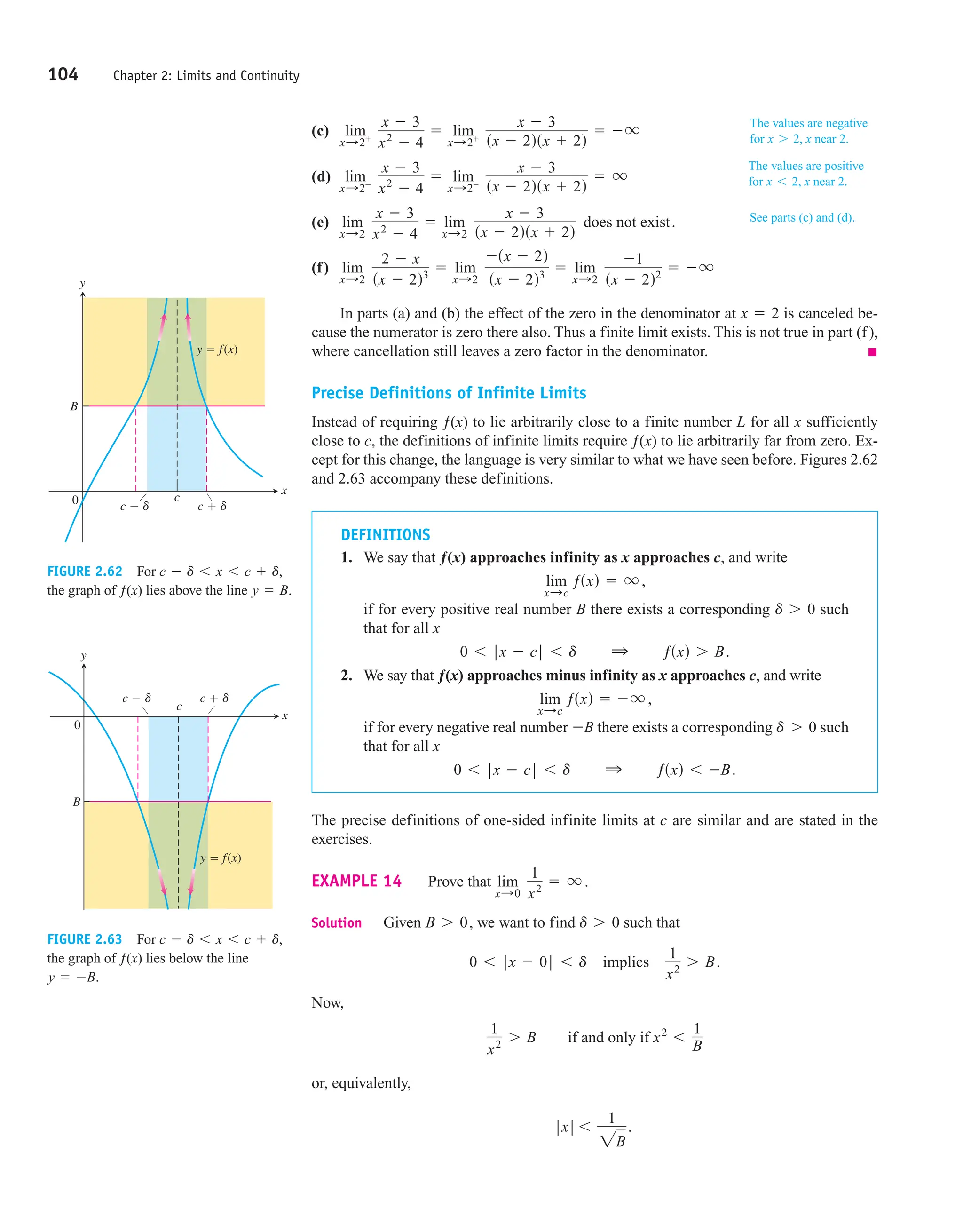


![114 Chapter 2: Limits and Continuity
A 1-L measuring cup (a), modeled as a right circular cylinder (b)
of radius
Precise Definition of Limit
In Exercises 7–10, use the formal definition of limit to prove that the
function is continuous at c.
7. 8.
9. 10.
11. Uniqueness of limits Show that a function cannot have two dif-
ferent limits at the same point. That is, if and
then
12. Prove the limit Constant Multiple Rule:
13. One-sided limits If and
find
a. b.
c. d.
14. Limits and continuity Which of the following statements are
true, and which are false? If true, say why; if false, give a coun-
terexample (that is, an example confirming the falsehood).
a. If exists but does not exist, then
does not exist.
b. If neither nor exists, then
does not exist.
c. If ƒ is continuous at x, then so is
d. If is continuous at c, then so is ƒ.
In Exercises 15 and 16, use the formal definition of limit to prove that
the function has a continuous extension to the given value of x.
15. 16. gsxd =
x2
- 2x - 3
2x - 6
, x = 3
ƒsxd =
x2
- 1
x + 1
, x = -1
ƒ ƒ ƒ
ƒ ƒ ƒ.
limx:c sƒsxd + gsxdd
limx:c gsxd
limx:c ƒsxd
limx:csƒsxd + gsxdd
limx:c gsxd
limx:c ƒsxd
limx:0- ƒsx2
- x4
d
limx:0+ ƒsx2
- x4
d
limx:0- ƒsx3
- xd
limx:0+ ƒsx3
- xd
limx:0- ƒsxd = B,
limx:0+ ƒsxd = A
lim
x:c
kƒsxd = k lim
x:c
ƒsxd for any constant k.
L1 = L2 .
limx:c ƒsxd = L2 ,
limx:c ƒsxd = L1
Fsxd = 29 - x, c = 5
hsxd = 22x - 3, c = 2
gsxd = 1s2xd, c = 14
ƒsxd = x2
- 7, c = 1
r = 6 cm
Stripes
about
1 mm
wide
r 6 cm
Liquid volume
V 36h
(a)
(b)
h
17. A function continuous at only one point Let
a. Show that ƒ is continuous at
b. Use the fact that every nonempty open interval of real num-
bers contains both rational and irrational numbers to show
that ƒ is not continuous at any nonzero value of x.
18. The Dirichlet ruler function If x is a rational number, then x
can be written in a unique way as a quotient of integers
where and m and n have no common factors greater than 1.
(We say that such a fraction is in lowest terms. For example,
written in lowest terms is .) Let ƒ(x) be defined for all x in the
interval [0, 1] by
For instance,
and so on.
a. Show that ƒ is discontinuous at every rational number in [0, 1].
b. Show that ƒ is continuous at every irrational number in [0, 1].
(Hint: If is a given positive number, show that there are only
finitely many rational numbers r in [0, 1] such that )
c. Sketch the graph of ƒ. Why do you think ƒ is called the “ruler
function”?
19. Antipodal points Is there any reason to believe that there is al-
ways a pair of antipodal (diametrically opposite) points on Earth’s
equator where the temperatures are the same? Explain.
20. If and find
21. Roots of a quadratic equation that is almost linear The equa-
tion where a is a constant, has two roots if
and one positive and one negative:
a. What happens to as As
b. What happens to as As
c. Support your conclusions by graphing and as
functions of a. Describe what you see.
d. For added support, graph simultane-
ously for and 0.05.
22. Root of an equation Show that the equation
has at least one solution.
23. Bounded functions A real-valued function ƒ is bounded from
above on a set D if there exists a number N such that
for all x in D. We call N, when it exists, an upper bound for ƒ on
D and say that ƒ is bounded from above by N. In a similar manner,
we say that ƒ is bounded from below on D if there exists a num-
ber M such that for all x in D. We call M, when it
exists, a lower bound for ƒ on D and say that ƒ is bounded from
below by M. We say that ƒ is bounded on D if it is bounded from
both above and below.
a. Show that ƒ is bounded on D if and only if there exists a num-
ber B such that for all x in D.
ƒ ƒsxd ƒ … B
ƒsxd Ú M
ƒsxd … N
x + 2 cos x = 0
a = 1, 0.5, 0.2, 0.1,
ƒsxd = ax2
+ 2x - 1
r-sad
r+sad
a : -1+
?
a : 0?
r-sad
a : -1+
?
a : 0?
r+sad
r+sad =
-1 + 21 + a
a , r-sad =
-1 - 21 + a
a .
a Z 0,
a 7 -1
ax2
+ 2x - 1 = 0,
lim
x:c
ƒsxdgsxd.
lim
x:c
sƒsxd - gsxdd = -1,
lim
x:c
sƒsxd + gsxdd = 3
ƒsrd Ú P.
P
ƒs14d = ƒs34d = 14,
13,
ƒs13d = ƒ(23) =
ƒs12d = 12,
ƒs0d = ƒs1d = 1,
ƒsxd = e
1n, if x = mn is a rational number in lowest terms
0, if x is irrational.
32
64
n 7 0
mn
x = 0.
ƒsxd = e
x, if x is rational
0, if x is irrational.](https://image.slidesharecdn.com/calculusbook-250617105057-211abae9/75/Complete-University-of-Calculus-2nd-edition-131-2048.jpg)


![EXAMPLE 3 Graph the derivative of the function in Figure 3.6a.
Solution We sketch the tangents to the graph of ƒ at frequent intervals and use their
slopes to estimate the values of at these points. We plot the corresponding
pairs and connect them with a smooth curve as sketched in Figure 3.6b.
What can we learn from the graph of At a glance we can see
1. where the rate of change of ƒ is positive, negative, or zero;
2. the rough size of the growth rate at any x and its size in relation to the size of ƒ(x);
3. where the rate of change itself is increasing or decreasing.
Differentiable on an Interval; One-Sided Derivatives
A function is differentiable on an open interval (finite or infinite) if it has a
derivative at each point of the interval. It is differentiable on a closed interval [a, b] if it
is differentiable on the interior (a, b) and if the limits
Right-hand derivative at a
Left-hand derivative at b
exist at the endpoints (Figure 3.7).
Right-hand and left-hand derivatives may be defined at any point of a function’s do-
main. Because of Theorem 6, Section 2.4, a function has a derivative at a point if and only if
it has left-hand and right-hand derivatives there, and these one-sided derivatives are equal.
EXAMPLE 4 Show that the function is differentiable on and
but has no derivative at
Solution From Section 3.1, the derivative of is the slope m. Thus, to the
right of the origin,
To the left,
(Figure 3.8). There is no derivative at the origin because the one-sided derivatives differ
there:
= lim
h:0-
-1 = -1.
= lim
h:0-
-h
h
Left-hand derivative of ƒ x ƒ at zero = lim
h:0-
ƒ 0 + h ƒ - ƒ 0 ƒ
h
= lim
h:0-
ƒ h ƒ
h
= lim
h:0+
1 = 1
= lim
h:0+
h
h
Right-hand derivative of ƒ x ƒ at zero = lim
h:0+
ƒ 0 + h ƒ - ƒ 0 ƒ
h
= lim
h:0+
ƒ h ƒ
h
ƒ x ƒ = -x
d
dx
sƒ x ƒd =
d
dx
s-xd =
d
dx
s-1 # xd = -1
ƒ x ƒ = x
d
dx
smx + bd = m,
d
dx
sƒ x ƒd =
d
dx
sxd =
d
dx
s1 # xd = 1.
y = mx + b
x = 0.
s0, qd
s- q, 0d
y = ƒ x ƒ
lim
h:0-
ƒsb + hd - ƒsbd
h
lim
h:0+
ƒsa + hd - ƒsad
h
y = ƒsxd
y = ƒ¿sxd?
sx, ƒ¿sxdd
ƒ¿sxd
y = ƒsxd
3.2 The Derivative as a Function 123
0 10
(a)
5 15
5
10
Slope 0
A
B
C
D
E
Slope 0
10
5 15
1
2
3
4
–1
–2
⎧
⎪
⎪
⎪
⎨
⎪
⎪
⎪
⎩
⎧
⎪
⎨
⎪
⎩
(b)
Slope –1
4
3
Slope
y f(x)
8
4 x-units
A'
y f '(x)
B'
C'
D'
E'
Vertical coordinate –1
y
x
x
Slope
–
FIGURE 3.6 We made the graph of
in (b) by plotting slopes from
the graph of in (a). The vertical
coordinate of is the slope at B and so on.
The slope at E is approximately
In (b) we see that the rate of change of ƒ is
negative for x between and the rate
of change is positive for x to the right of D¿.
D¿;
A¿
84 = 2.
B¿
y = ƒsxd
y = ƒ¿sxd
a b
a h
h 0
b h
h 0
lim
h→0
f(a h) f(a)
h
Slope
y f(x)
lim
h→0
f(b h) f(b)
h
Slope
x
FIGURE 3.7 Derivatives at endpoints are
one-sided limits.
ƒ h ƒ = h when h 7 0
ƒ h ƒ = -h when h 6 0](https://image.slidesharecdn.com/calculusbook-250617105057-211abae9/75/Complete-University-of-Calculus-2nd-edition-140-2048.jpg)


![126 Chapter 3: Differentiation
Slopes and Tangent Lines
In Exercises 13–16, differentiate the functions and find the slope of
the tangent line at the given value of the independent variable.
13. 14.
15. 16.
In Exercises 17–18, differentiate the functions. Then find an equation
of the tangent line at the indicated point on the graph of the function.
17.
18.
In Exercises 19–22, find the values of the derivatives.
19.
20.
21.
22.
Using the Alternative Formula for Derivatives
Use the formula
to find the derivative of the functions in Exercises 23–26.
23. 24.
25. 26.
Graphs
Match the functions graphed in Exercises 27–30 with the derivatives
graphed in the accompanying figures (a)–(d).
y'
0
x
(d)
y'
0
x
(c)
y'
0
x
(a)
y'
0
x
(b)
gsxd = 1 + 1x
gsxd =
x
x - 1
ƒsxd = x2
- 3x + 4
ƒsxd =
1
x + 2
ƒ¿sxd = lim
z:x
ƒszd - ƒsxd
z - x
dw
dz
`
z=4
if w = z + 1z
dr
du
`
u=0
if r =
2
24 - u
dy
dx
`
x= 23
if y = 1 -
1
x
ds
dt
`
t= -1
if s = 1 - 3t2
w = gszd = 1 + 24 - z, sz, wd = s3, 2d
y = ƒsxd =
8
2x - 2
, sx, yd = s6, 4d
y =
x + 3
1 - x
, x = -2
s = t3
- t2
, t = -1
ksxd =
1
2 + x
, x = 2
ƒsxd = x +
9
x , x = -3
27. 28.
29. 30.
31. a. The graph in the accompanying figure is made of line seg-
ments joined end to end. At which points of the interval
is not defined? Give reasons for your answer.
b. Graph the derivative of ƒ.
The graph should show a step function.
32. Recovering a function from its derivative
a. Use the following information to graph the function ƒ over
the closed interval
i) The graph of ƒ is made of closed line segments joined
end to end.
ii) The graph starts at the point
iii) The derivative of ƒ is the step function in the figure
shown here.
b. Repeat part (a), assuming that the graph starts at
instead of s -2, 3d.
s-2, 0d
x
0 1
–2 3 5
1
y'
y' f'(x)
–2
s-2, 3d.
[-2, 5].
x
y
0 1 6
(0, 2) (6, 2)
(–4, 0)
y f(x)
(4, –2)
(1, –2)
ƒ¿
[-4, 6]
y
0
x
y f4(x)
y
0
x
y f3(x)
x
y
0
y f2(x)
x
y
0
y f1(x)](https://image.slidesharecdn.com/calculusbook-250617105057-211abae9/75/Complete-University-of-Calculus-2nd-edition-143-2048.jpg)


![Proof
Constant Multiple Limit Property
u is differentiable.
EXAMPLE 2
(a) The derivative formula
says that if we rescale the graph of by multiplying each y-coordinate by 3, then
we multiply the slope at each point by 3 (Figure 3.10).
(b) Negative of a function
The derivative of the negative of a differentiable function u is the negative of the func-
tion’s derivative. The Constant Multiple Rule with gives
The next rule says that the derivative of the sum of two differentiable functions is the
sum of their derivatives.
d
dx
s-ud =
d
dx
s-1 # ud = -1 # d
dx
sud = -
du
dx
.
c = -1
y = x2
d
dx
s3x2
d = 3 # 2x = 6x
= c
du
dx
= c lim
h:0
usx + hd - usxd
h
d
dx
cu = lim
h:0
cusx + hd - cusxd
h
3.3 Differentiation Rules 131
x
y
0 1
1
(1, 1)
2
2
3 (1, 3) Slope
Slope
Slope 2x
2(1) 2
y x2
y 3x2
Slope 3(2x)
6x
6(1) 6
FIGURE 3.10 The graphs of and
Tripling the y-coordinate triples
the slope (Example 2).
y = 3x2
.
y = x2
For example, if , then y is the sum of and We
then have
Proof We apply the definition of the derivative to
Combining the Sum Rule with the Constant Multiple Rule gives the Difference Rule,
which says that the derivative of a difference of differentiable functions is the difference of
their derivatives:
d
dx
su - yd =
d
dx
[u + s-1dy] =
du
dx
+ s-1d
dy
dx
=
du
dx
-
dy
dx
.
= lim
h:0
usx + hd - usxd
h
+ lim
h:0
ysx + hd - ysxd
h
=
du
dx
+
dy
dx
.
= lim
h:0
c
usx + hd - usxd
h
+
ysx + hd - ysxd
h
d
d
dx
[usxd + ysxd] = lim
h:0
[usx + hd + ysx + hd] - [usxd + ysxd]
h
ƒsxd = usxd + ysxd:
dy
dx
=
d
dx
(x4
) +
d
dx
(12x) = 4x3
+ 12.
y(x) = 12x.
u(x) = x4
y = x4
+ 12x
Derivative definition
with ƒsxd = cusxd
Derivative Sum Rule
If u and are differentiable functions of x, then their sum is differentiable
at every point where u and are both differentiable. At such points,
d
dx
su + yd =
du
dx
+
dy
dx
.
y
u + y
y
Denoting Functions by u and
The functions we are working with when
we need a differentiation formula are
likely to be denoted by letters like ƒ and g.
We do not want to use these same letters
when stating general differentiation rules,
so instead we use letters like u and that
are not likely to be already in use.
y
Y](https://image.slidesharecdn.com/calculusbook-250617105057-211abae9/75/Complete-University-of-Calculus-2nd-edition-148-2048.jpg)


![134 Chapter 3: Differentiation
Products and Quotients
While the derivative of the sum of two functions is the sum of their derivatives, the deriva-
tive of the product of two functions is not the product of their derivatives. For instance,
The derivative of a product of two functions is the sum of two products, as we now explain.
d
dx
sx # xd =
d
dx
sx2
d = 2x, while
d
dx
sxd # d
dx
sxd = 1 # 1 = 1.
Derivative Product Rule
If u and are differentiable at x, then so is their product u , and
d
dx
suyd = u
dy
dx
+ y
du
dx
.
y
y
The derivative of the product u is u times the derivative of plus times the deriva-
tive of u. In prime notation, In function notation,
EXAMPLE 6 Find the derivative of (a) , (b)
Solution
(a) We apply the Product Rule with and
(b)
Proof of the Derivative Product Rule
To change this fraction into an equivalent one that contains difference quotients for the de-
rivatives of u and , we subtract and add in the numerator:
As h approaches zero, approaches u(x) because u, being differentiable at x, is con-
tinuous at x. The two fractions approach the values of at x and at x. In short,
d
dx
suyd = u
dy
dx
+ y
du
dx
.
dudx
dydx
usx + hd
= lim
h:0
usx + hd # lim
h:0
ysx + hd - ysxd
h
+ ysxd # lim
h:0
usx + hd - usxd
h
.
= lim
h:0
cusx + hd
ysx + hd - ysxd
h
+ ysxd
usx + hd - usxd
h
d
d
dx
suyd = lim
h:0
usx + hdysx + hd - usx + hdysxd + usx + hdysxd - usxdysxd
h
usx + hdysxd
y
d
dx
suyd = lim
h:0
usx + hdysx + hd - usxdysxd
h
d
dx
(e2x
) =
d
dx
(ex # ex
) = ex # d
dx
(ex
) + ex # d
dx
(ex
) = 2ex # ex
= 2e2x
= 1 + (x - 1)
ex
x2
.
= 2 +
ex
x - 1 -
ex
x2
d
dx
c
1
x Ax2
+ ex
B d =
1
x A2x + ex
B + Ax2
+ ex
B a-
1
x2
b
y = x2
+ ex
:
u = 1x
y = e2x
.
y =
1
x Ax2
+ ex
B
d
dx
[ƒsxdgsxd] = ƒsxdg¿sxd + gsxdƒ¿sxd.
suyd¿ = uy¿ + yu¿.
y
y
y
d
dx
a
1
x b = -
1
x2
d
dx
suyd = u
dy
dx
+ y
du
dx
, and
0
y(x h)
y(x)
y
u(x)y(x)
u(x h) y
y(x) u
u(x h)
u(x)
u
Then the change in the product uy is the
difference in areas of the larger and
smaller “squares,” which is the sum of the
upper and right-hand reddish-shaded
rectangles. That is,
Division by h gives
The limit as gives the Product
Rule.
h : 0+
¢(uy)
h
= u(x + h)
¢y
h
+ y(x)
¢u
h
.
= u(x + h)¢y + y(x)¢u.
¢(uy) = u(x + h)y(x + h) - u(x)y(x)
Picturing the Product Rule
Suppose u(x) and (x) are positive and
increase when x increases, and h 7 0.
y](https://image.slidesharecdn.com/calculusbook-250617105057-211abae9/75/Complete-University-of-Calculus-2nd-edition-151-2048.jpg)


![59. By computing the first few derivatives and looking for a pattern,
find
60. Derive the formula for the derivative with respect to x of
a. sec x. b. csc x. c. cot x.
61. A weight is attached to a spring and reaches its equilibrium posi-
tion It is then set in motion resulting in a displacement of
where x is measured in centimeters and t is measured in seconds.
See the accompanying figure.
a. Find the spring’s displacement when and
b. Find the spring’s velocity when and
62. Assume that a particle’s position on the x-axis is given by
where x is measured in feet and t is measured in seconds.
a. Find the particle’s position when and
b. Find the particle’s velocity when and
63. Graph for On the same screen, graph
for and 0.1. Then, in a new window, try
and What happens as As
What phenomenon is being illustrated here?
64. Graph for On the same screen, graph
for and 0.1. Then, in a new window, try
and What happens as As
What phenomenon is being illustrated here?
65. Centered difference quotients The centered difference quotient
is used to approximate in numerical work because (1) its
limit as equals when exists, and (2) it usually
gives a better approximation of for a given value of h than
the difference quotient
ƒsx + hd - ƒsxd
h
.
ƒ¿sxd
ƒ¿sxd
ƒ¿sxd
h : 0
ƒ¿sxd
ƒsx + hd - ƒsx - hd
2h
h : 0-
?
h : 0+
?
-0.3.
h = -1, -0.5,
h = 1, 0.5, 0.3,
y =
cossx + hd - cos x
h
-p … x … 2p.
y = -sin x
h : 0-
?
h : 0+
?
-0.3.
h = -1, -0.5,
h = 1, 0.5, 0.3,
y =
sinsx + hd - sin x
h
-p … x … 2p.
y = cos x
t = p.
t = 0, t = p2,
t = p.
t = 0, t = p2,
x = 3 cos t + 4 sin t,
t = 3p4.
t = 0, t = p3,
t = 3p4.
t = 0, t = p3,
x
0
–10
10
Equilibrium
position
at x 5 0
x = 10 cos t,
sx = 0d.
d999
dx999
scos xd.
3.5 Derivatives of Trigonometric Functions 155
See the accompanying figure.
a. To see how rapidly the centered difference quotient for
converges to graph
together with
over the interval for and 0.3. Compare
the results with those obtained in Exercise 63 for the same
values of h.
b. To see how rapidly the centered difference quotient for
converges to graph
together with
over the interval and 0.3. Compare
the results with those obtained in Exercise 64 for the same
values of h.
66. A caution about centered difference quotients (Continuation
of Exercise 65.) The quotient
may have a limit as when ƒ has no derivative at x. As a case
in point, take and calculate
As you will see, the limit exists even though has no de-
rivative at Moral: Before using a centered difference quo-
tient, be sure the derivative exists.
67. Slopes on the graph of the tangent function Graph
and its derivative together on Does the graph of the
tangent function appear to have a smallest slope? A largest slope?
Is the slope ever negative? Give reasons for your answers.
s-p2, p2d.
y = tan x
x = 0.
ƒsxd = ƒ x ƒ
lim
h:0
ƒ 0 + h ƒ - ƒ 0 - h ƒ
2h
.
ƒsxd = ƒ x ƒ
h : 0
ƒsx + hd - ƒsx - hd
2h
[-p, 2p] for h = 1, 0.5,
y =
cossx + hd - cossx - hd
2h
y = -sin x
ƒ¿sxd = -sin x,
ƒsxd = cos x
h = 1, 0.5,
[-p, 2p]
y =
sinsx + hd - sinsx - hd
2h
y = cos x
ƒ¿sxd = cos x,
ƒsxd = sin x
x
y
0 x
A
h
h
C
B
x h x h
y f(x)
Slope f'(x)
Slope
Slope
h
f(x h) f(x)
f(x h) f(x h)
2h
T
T
T
T](https://image.slidesharecdn.com/calculusbook-250617105057-211abae9/75/Complete-University-of-Calculus-2nd-edition-172-2048.jpg)


![b. Can anything be said about the tangents to the curves
and at the origin
Give reasons for your answer.
c. For a given m, what are the largest values the slopes of the
curves and can ever have? Give
reasons for your answer.
d. The function completes one period on the interval
the function completes two periods, the
function completes half a period, and so on. Is
there any relation between the number of periods
completes on and the slope of the curve
at the origin? Give reasons for your answer.
97. Running machinery too fast Suppose that a piston is moving
straight up and down and that its position at time t sec is
with A and b positive. The value of A is the amplitude of the mo-
tion, and b is the frequency (number of times the piston moves up
and down each second). What effect does doubling the frequency
have on the piston’s velocity, acceleration, and jerk? (Once you
find out, you will know why some machinery breaks when you
run it too fast.)
98. Temperatures in Fairbanks,Alaska The graph in the accom-
panying figure shows the average Fahrenheit temperature in
Fairbanks, Alaska, during a typical 365-day year. The equation
that approximates the temperature on day x is
and is graphed in the accompanying figure.
a. On what day is the temperature increasing the fastest?
b. About how many degrees per day is the temperature increas-
ing when it is increasing at its fastest?
99. Particle motion The position of a particle moving along a co-
ordinate line is with s in meters and t in seconds.
Find the particle’s velocity and acceleration at
100. Constant acceleration Suppose that the velocity of a falling
body is (k a constant) at the instant the body
has fallen s m from its starting point. Show that the body’s accel-
eration is constant.
101. Falling meteorite The velocity of a heavy meteorite entering
Earth’s atmosphere is inversely proportional to when it is
s km from Earth’s center. Show that the meteorite’s acceleration
is inversely proportional to s2
.
1s
y = k1s msec
t = 6 sec.
s = 21 + 4t,
J
a
n
F
e
b
M
a
r
A
p
r
M
a
y
J
u
n
J
u
l
A
u
g
S
e
p
O
c
t
N
o
v
D
e
c
J
a
n
F
e
b
M
a
r
0
–20
20
40
60
x
y
.......
. .
.
..
.....
.
. ..... ....
.
.
.
.
..........
......
....... ..... .....
..
...
......
.........
.
....
............
....
.
..
...
.........
..... .........
....
Temperature
(˚F)
y = 37 sin c
2p
365
sx - 101dd + 25
s = A coss2pbtd,
y = sin mx
[0, 2p]
y = sin mx
y = sinsx2d
y = sin 2x
[0, 2p],
y = sin x
y = -sinsxmd
y = sin mx
sm a constant Z 0d?
y = -sinsxmd
y = sin mx
3.6 The Chain Rule 163
102. Particle acceleration A particle moves along the x-axis with
velocity Show that the particle’s acceleration is
103. Temperature and the period of a pendulum For oscillations
of small amplitude (short swings), we may safely model the rela-
tionship between the period T and the length L of a simple pen-
dulum with the equation
where g is the constant acceleration of gravity at the pendulum’s lo-
cation. If we measure g in centimeters per second squared, we
measure L in centimeters and T in seconds. If the pendulum is made
of metal, its length will vary with temperature, either increasing or
decreasing at a rate that is roughly proportional to L. In symbols,
with u being temperature and k the proportionality constant,
Assuming this to be the case, show that the rate at which the pe-
riod changes with respect to temperature is .
104. Chain Rule Suppose that and Then the
composites
are both differentiable at even though g itself is not differ-
entiable at Does this contradict the Chain Rule? Explain.
105. The derivative of sin 2x Graph the function for
Then, on the same screen, graph
for and 0.2. Experiment with other values of h, in-
cluding negative values. What do you see happening as
Explain this behavior.
106. The derivative of Graph for
Then, on the same screen, graph
for Experiment with other values of h.
What do you see happening as Explain this behavior.
Using the Chain Rule, show that the Power Rule
holds for the functions in Exercises 107 and 108.
107. 108.
COMPUTER EXPLORATIONS
Trigonometric Polynomials
109. As the accompanying figure shows, the trigonometric “polynomial”
gives a good approximation of the sawtooth function
on the interval How well does the derivative of ƒ ap-
proximate the derivative of g at the points where is de-
fined? To find out, carry out the following steps.
dgdt
[-p, p].
s = gstd
- 0.02546 cos 10t - 0.01299 cos 14t
s = ƒstd = 0.78540 - 0.63662 cos 2t - 0.07074 cos 6t
x34
= 2x1x
x14
= 21x
xn
sddxdxn
= nxn-1
h : 0?
h = 1.0, 0.7, and 0.3.
y =
cos ssx + hd2
d - cos sx2
d
h
-2 … x … 3.
y = -2x sin sx2
d
cos sx2
d
h : 0?
h = 1.0, 0.5,
y =
sin 2sx + hd - sin 2x
h
-2 … x … 3.5.
y = 2 cos 2x
x = 0.
x = 0
sƒ ⴰ gdsxd = ƒ x ƒ
2
= x2
and sg ⴰ ƒdsxd = ƒ x2
ƒ = x2
gsxd = ƒ x ƒ.
ƒsxd = x2
kT2
dL
du
= kL.
T = 2p
A
L
g ,
ƒsxdƒ¿sxd.
dxdt = ƒsxd.
T](https://image.slidesharecdn.com/calculusbook-250617105057-211abae9/75/Complete-University-of-Calculus-2nd-edition-180-2048.jpg)
![a. Graph (where defined) over
b. Find .
c. Graph . Where does the approximation of by
seem to be best? Least good? Approximations by
trigonometric polynomials are important in the theories of
heat and oscillation, but we must not expect too much of
them, as we see in the next exercise.
110. (Continuation of Exercise 109.) In Exercise 109, the trigonometric
polynomial that approximated the sawtooth function g(t) on
had a derivative that approximated the derivative of the
sawtooth function. It is possible, however, for a trigonometric
polynomial to approximate a function in a reasonable way with-
out its derivative approximating the function’s derivative at all
well. As a case in point, the “polynomial”
[-p, p]
ƒ(t)
t
s
0
–
2
s g(t)
s f(t)
dƒdt
dgdt
dƒdt
dƒdt
[-p, p].
dgdt
164 Chapter 3: Differentiation
x
y
0 5
5
A
x3
y3
9xy 0
y f1(x)
(x0, y1)
y f2(x)
y f3(x)
(x0, y2)
(x0, y3)
x0
FIGURE 3.28 The curve
is not the graph of
any one function of x. The curve can,
however, be divided into separate arcs that
are the graphs of functions of x. This
particular curve, called a folium, dates to
Descartes in 1638.
x3
+ y3
- 9xy = 0
graphed in the accompanying figure approximates the step func-
tion shown there. Yet the derivative of h is nothing like
the derivative of k.
a. Graph (where defined) over
b. Find
c. Graph to see how badly the graph fits the graph of
. Comment on what you see.
dkdt
dhdt
dhdt.
[-p, p].
dkdt
1
t
s
0
2
–
2
–
–1
s k(t)
s h(t)
s = kstd
+ 0.18189 sin 14t + 0.14147 sin 18t
s = hstd = 1.2732 sin 2t + 0.4244 sin 6t + 0.25465 sin 10t
3.7
Implicit Differentiation
Most of the functions we have dealt with so far have been described by an equation of the
form that expresses y explicitly in terms of the variable x. We have learned rules
for differentiating functions defined in this way. Another situation occurs when we en-
counter equations like
(See Figures 3.28, 3.29, and 3.30.) These equations define an implicit relation between the
variables x and y. In some cases we may be able to solve such an equation for y as an ex-
plicit function (or even several functions) of x. When we cannot put an equation
in the form to differentiate it in the usual way, we may still be able
to find by implicit differentiation. This section describes the technique.
Implicitly Defined Functions
We begin with examples involving familiar equations that we can solve for y as a function
of x to calculate in the usual way. Then we differentiate the equations implicitly, and
find the derivative to compare the two methods. Following the examples, we summarize
the steps involved in the new method. In the examples and exercises, it is always assumed
that the given equation determines y implicitly as a differentiable function of x so that
exists.
EXAMPLE 1 Find if
Solution The equation defines two differentiable functions of x that we can actu-
ally find, namely and (Figure 3.29). We know how to calculate the
derivative of each of these for
dy1
dx
=
1
21x
and
dy2
dx
= -
1
21x
.
x 7 0:
y2 = - 1x
y1 = 1x
y2
= x
y2
= x.
dydx
dydx
dydx
dydx
y = ƒsxd
Fsx, yd = 0
x3
+ y3
- 9xy = 0, y2
- x = 0, or x2
+ y2
- 25 = 0.
y = ƒsxd](https://image.slidesharecdn.com/calculusbook-250617105057-211abae9/75/Complete-University-of-Calculus-2nd-edition-181-2048.jpg)
![But suppose that we knew only that the equation defined y as one or more differ-
entiable functions of x for without knowing exactly what these functions were.
Could we still find ?
The answer is yes. To find , we simply differentiate both sides of the equation
with respect to x, treating as a differentiable function of x:
This one formula gives the derivatives we calculated for both explicit solutions
and
EXAMPLE 2 Find the slope of the circle at the point
Solution The circle is not the graph of a single function of x. Rather, it is the combined
graphs of two differentiable functions, and (Figure
3.30). The point lies on the graph of so we can find the slope by calculating the
derivative directly, using the Power Chain Rule:
We can solve this problem more easily by differentiating the given equation of the
circle implicitly with respect to x:
The slope at is
Notice that unlike the slope formula for which applies only to points
below the x-axis, the formula applies everywhere the circle has a slope.
Notice also that the derivative involves both variables x and y, not just the independent
variable x.
To calculate the derivatives of other implicitly defined functions, we proceed as in
Examples 1 and 2: We treat y as a differentiable implicit function of x and apply the usual
rules to differentiate both sides of the defining equation.
dydx = -xy
dy2dx,
-
x
y `
s3, -4d
= -
3
-4
=
3
4
.
s3, -4d
dy
dx
= -
x
y .
2x + 2y
dy
dx
= 0
d
dx
(x2
) +
d
dx
(y2
) =
d
dx
(25)
dy2
dx
`
x=3
= -
-2x
2225 - x2
`
x=3
= -
-6
2225 - 9
=
3
4
.
y2,
s3, -4d
y2 = - 225 - x2
y1 = 225 - x2
s3, -4d.
x2
+ y2
= 25
dy1
dx
=
1
2y1
=
1
21x
and
dy2
dx
=
1
2y2
=
1
2A - 1xB
= -
1
21x
.
y2 = - 1x:
y1 = 1x
dy
dx
=
1
2y
.
2y
dy
dx
= 1
y2
= x
y = ƒsxd
y2
= x
dydx
dydx
x 7 0
y2
= x
3.7 Implicit Differentiation 165
x
y
0
y2
x
Slope
2y1
1
2x
1
Slope
2y2
1
2x
1
y1 x
y2 x
P(x, x)
Q(x, x )
FIGURE 3.29 The equation
or as it is usually written, defines
two differentiable functions of x on the
interval Example 1 shows how to
find the derivatives of these functions
without solving the equation for y.
y2
= x
x 7 0.
y2
= x
y2
- x = 0,
-
1
2
(25 - x2
)-12
(-2x)
d
dx
a-(25 - x2
)12
b =
The Chain Rule gives
d
dx
[ƒsxd]
2
= 2ƒsxdƒ¿sxd = 2y
dy
dx
.
d
dx
Ay2
B =
0 5
–5
x
y
Slope –
y
x
4
3
(3, –4)
y1 25 x2
y2 –25 x2
FIGURE 3.30 The circle combines the
graphs of two functions. The graph of is
the lower semicircle and passes through
s3, -4d.
y2](https://image.slidesharecdn.com/calculusbook-250617105057-211abae9/75/Complete-University-of-Calculus-2nd-edition-182-2048.jpg)


![We use open or half-open intervals when describing the ranges to avoid values where the
tangent, cotangent, secant, and cosecant functions are undefined. (See Figure 3.40.)
The graph of is symmetric about the origin because it is a branch of the
graph that is symmetric about the origin (Figure 3.40a). Algebraically this
means that
the arctangent is an odd function. The graph of has no such symmetry
(Figure 3.40b). Notice from Figure 3.40a that the graph of the arctangent function has two
horizontal asymptotes; one at and the other at .
y = -p2
y = p2
y = cot-1
x
tan-1
s-xd = -tan-1
x;
x = tan y
y = tan-1
x
3.9 Inverse Trigonometric Functions
We introduced the six basic inverse trigonometric functions in Section 1.6, but focused
there on the arcsine and arccosine functions. Here we complete the study of how all six in-
verse trigonometric functions are defined, graphed, and evaluated, and how their deriva-
tives are computed.
Inverses of and
The graphs of these four basic inverse trigonometric functions are shown again in Figure 3.40.
We obtain these graphs by reflecting the graphs of the restricted trigonometric functions
(as discussed in Section 1.6) through the line Let’s take a closer look at the arctan-
gent, arccotangent, arcsecant, and arccosecant functions.
y = x.
csc x
tan x, cot x, sec x,
180 Chapter 3: Differentiation
x
y
(a)
Domain:
Range:
–∞ x ∞
y
2
–
2
1
–1
–2 2
2
2
–
y tan–1
x
x
y
(c)
Domain:
Range:
x –1 or x 1
0 y , y
1
–1
–2 2
y sec–1
x
2
2
x
y
Domain:
Range:
x –1 or x 1
y , y 0
2
–
2
(d)
1
–1
–2 2
2
2
–
y csc–1
x
x
y
Domain:
Range: 0 y
(b)
2
1
–1
–2 2
y cot–1
x
–∞ x ∞
FIGURE 3.40 Graphs of the arctangent, arccotangent, arcsecant, and arccosecant functions.
DEFINITION
is the number in for which sec
y csc1
x is the number in [-p/2, 0) ´ (0, p/2] for which csc y = x.
y = x.
[0, p/2) ´ (p/2, p]
y sec1
x
y cot1
x is the number in s0, pd for which cot y = x.
y tan1
x is the number in s-p2, p2d for which tan y = x.
The arctangent of x is a radian angle whose tangent is x. The arccotangent of x is an angle
whose cotangent is x, and so forth. The angles belong to the restricted domains of the tangent,
cotangent, secant, and cosecant functions.](https://image.slidesharecdn.com/calculusbook-250617105057-211abae9/75/Complete-University-of-Calculus-2nd-edition-197-2048.jpg)


![An important linear approximation for roots and powers is
(Exercise 15). This approximation, good for values of x sufficiently close to zero, has
broad application. For example, when x is small,
Differentials
We sometimes use the Leibniz notation to represent the derivative of y with respect
to x. Contrary to its appearance, it is not a ratio. We now introduce two new variables dx
and dy with the property that when their ratio exists, it is equal to the derivative.
dydx
1
21 - x2
= s1 - x2
d-12
L 1 + a-
1
2
bs-x2
d = 1 +
1
2
x2
k = 13; replace x by 5x4
.
2
3
1 + 5x4
= s1 + 5x4
d13
L 1 +
1
3
s5x4
d = 1 +
5
3
x4
k = -1; replace x by -x.
1
1 - x
= s1 - xd-1
L 1 + s-1ds -xd = 1 + x
k = 12
21 + x L 1 +
1
2
x
s1 + xdk
L 1 + kx sx near 0; any number kd
198 Chapter 3: Differentiation
replace x by -x2
.
k = -12;
DEFINITION Let be a differentiable function. The differential dx is
an independent variable. The differential dy is
dy = ƒ¿sxd dx.
y = ƒsxd
Unlike the independent variable dx, the variable dy is always a dependent variable. It
depends on both x and dx. If dx is given a specific value and x is a particular number in the
domain of the function ƒ, then these values determine the numerical value of dy.
EXAMPLE 4
(a) Find dy if
(b) Find the value of dy when and
Solution
(a)
(b) Substituting and in the expression for dy, we have
The geometric meaning of differentials is shown in Figure 3.55. Let and set
The corresponding change in is
The corresponding change in the tangent line L is
= ƒ¿(a) dx.
= ƒ(a) + ƒ¿(a)[(a + dx) - a] - ƒ(a)
¢L = L(a + dx) - L(a)
¢y = ƒsa + dxd - ƒsad.
y = ƒsxd
dx = ¢x.
x = a
dy = s5 # 14
+ 37d0.2 = 8.4.
dx = 0.2
x = 1
dy = s5x4
+ 37d dx
dx = 0.2.
x = 1
y = x5
+ 37x.
(++++++)++++++*
L(a dx)
()*
L(a)](https://image.slidesharecdn.com/calculusbook-250617105057-211abae9/75/Complete-University-of-Calculus-2nd-edition-215-2048.jpg)


![3.11 Linearization and Differentials 201
To estimate we set and Then
For comparison, the true value of to 6 decimals is 0.508635.
The method in part (b) of Example 7 is used by some calculator and computer algo-
rithms to give values of trigonometric functions. The algorithms store a large table of sine
and cosine values between 0 and Values between these stored values are computed
using differentials as in Example 7b. Values outside of are computed from values in
this interval using trigonometric identities.
Error in Differential Approximation
Let ƒ(x) be differentiable at and suppose that is an increment of x. We
have two ways to describe the change in ƒ as x changes from a to
How well does dƒ approximate
We measure the approximation error by subtracting dƒ from
As the difference quotient
approaches (remember the definition of ), so the quantity in parentheses be-
comes a very small number (which is why we called it ). In fact, as When
is small, the approximation error is smaller still.
Although we do not know the exact size of the error, it is the product of two small
quantities that both approach zero as For many common functions, whenever
is small, the error is still smaller.
¢x
¢x : 0.
P # ¢x
¢ƒ = ƒ¿(a)¢x + P ¢x
P ¢x
¢x
¢x : 0.
P : 0
P
ƒ¿sad
ƒ¿sad
ƒsa + ¢xd - ƒsad
¢x
¢x : 0,
= P # ¢x.
= a
ƒ(a + ¢x) - ƒ(a)
¢x
- ƒ¿(a)b # ¢x
= ƒ(a + ¢x) - ƒ(a) - ƒ¿(a)¢x
= ¢ƒ - ƒ¿sad¢x
Approximation error = ¢ƒ - dƒ
¢ƒ:
¢ƒ?
The differential estimate: dƒ = ƒ¿sad ¢x.
The true change: ¢ƒ = ƒsa + ¢xd - ƒsad
a + ¢x:
dx = ¢x
x = a
[0, p4]
p4.
sin (p6 + 0.01)
=
1
2
+
23
2
(0.01) L 0.5087
= sin
p
6
+ acos
p
6
b (0.01)
f (p6 + 0.01) = f (a + dx) L f (a) + dy
dx = 0.01.
a = p6
sin (p6 + 0.01),
(++++)++++*
ƒ
(+++++++)+++++++*
Call this part .
P
()*
true
change
(+)+*
estimated
change
()*
error](https://image.slidesharecdn.com/calculusbook-250617105057-211abae9/75/Complete-University-of-Calculus-2nd-edition-218-2048.jpg)


![where W is the work per unit time, P is the average blood pres-
sure, V is the volume of blood pumped out during the unit of time,
(“delta”) is the weight density of the blood, is the average ve-
locity of the exiting blood, and g is the acceleration of gravity.
When and remain constant, W becomes a function
of g, and the equation takes the simplified form
As a member of NASA’s medical team, you want to know how sen-
sitive W is to apparent changes in g caused by flight maneuvers,
and this depends on the initial value of g. As part of your investiga-
tion, you decide to compare the effect on W of a given change dg on
the moon, where with the effect the same change
dg would have on Earth, where Use the simplified
equation above to find the ratio of to
62. Measuring acceleration of gravity When the length L of a
clock pendulum is held constant by controlling its temperature,
the pendulum’s period T depends on the acceleration of gravity g.
The period will therefore vary slightly as the clock is moved from
place to place on the earth’s surface, depending on the change in g.
By keeping track of we can estimate the variation in g from the
equation that relates T, g, and L.
a. With L held constant and g as the independent variable,
calculate dT and use it to answer parts (b) and (c).
b. If g increases, will T increase or decrease? Will a pendulum
clock speed up or slow down? Explain.
c. A clock with a 100-cm pendulum is moved from a location
where to a new location. This increases the
period by Find dg and estimate the value of
g at the new location.
63. The linearization is the best linear approximation Suppose
that is differentiable at and that
is a linear function in which m and c are constants.
If the error were small enough near
we might think of using g as a linear approximation of ƒ instead
of the linearization Show that if we
impose on g the conditions
1. The approximation error is zero at
2.
then Thus, the linearization L(x)
gives the only linear approximation whose error is both zero at
and negligible in comparison with
64. Quadratic approximations
a. Let be a quadratic
approximation to ƒ(x) at with the properties:
i)
ii)
iii) Q–sad = ƒ–sad.
Q¿sad = ƒ¿sad
Qsad = ƒsad
x = a
Qsxd = b0 + b1sx - ad + b2sx - ad2
x
a
y f(x)
(a, f(a))
The linearization, L(x):
y f(a) f'(a)(x a)
Some other linear
approximation, g(x):
y m(x a) c
x - a.
x = a
gsxd = ƒsad + ƒ¿sadsx - ad.
lim
x:a
Esxd
x - a = 0
x = a.
Esad = 0
Lsxd = ƒsad + ƒ¿sadsx - ad.
x = a,
Esxd = ƒsxd - gsxd
msx - ad + c
gsxd =
x = a
y = ƒsxd
dT = 0.001 sec.
g = 980 cmsec2
T = 2psLgd12
¢T,
dWEarth .
dWmoon
g = 32 ftsec2
.
g = 5.2 ftsec2
,
W = a +
b
g sa, b constantd.
y
P, V, d,
y
d
3.11 Linearization and Differentials 205
Determine the coefficients and
b. Find the quadratic approximation to at
c. Graph and its quadratic approximation at
Then zoom in on the two graphs at the point (0, 1).
Comment on what you see.
d. Find the quadratic approximation to at
Graph g and its quadratic approximation together. Comment
on what you see.
e. Find the quadratic approximation to at
Graph h and its quadratic approximation together.
Comment on what you see.
f. What are the linearizations of ƒ, g, and h at the respective
points in parts (b), (d), and (e)?
65. The linearization of
a. Find the linearization of at Then round its
coefficients to two decimal places.
b. Graph the linearization and function together for
and
66. The linearization of
a. Find the linearization of at Then round
its coefficients to two decimal places.
b. Graph the linearization and function together in the window
and
COMPUTER EXPLORATIONS
In Exercises 67–72, use a CAS to estimate the magnitude of the error
in using the linearization in place of the function over a specified in-
terval I. Perform the following steps:
a. Plot the function ƒ over I.
b. Find the linearization L of the function at the point a.
c. Plot ƒ and L together on a single graph.
d. Plot the absolute error and find its
maximum value.
e. From your graph in part (d), estimate as large a as you
can, satisfying
for Then check graphically to see if
your holds true.
67.
68.
69.
70.
71.
72. ƒ(x) = 2x sin-1
x, [0, 1], a =
1
2
ƒ(x) = x2x
, [0, 2], a = 1
ƒsxd = 1x - sin x, [0, 2p], a = 2
ƒsxd = x23
sx - 2d, [-2, 3], a = 2
ƒsxd =
x - 1
4x2
+ 1
, c-
3
4
, 1d, a =
1
2
ƒsxd = x3
+ x2
- 2x, [-1, 2], a = 1
d-estimate
P = 0.5, 0.1, and 0.01.
ƒ x - a ƒ 6 d Q ƒ ƒsxd - Lsxd ƒ 6 P
d 7 0
ƒ ƒsxd - Lsxd ƒ over I
2 … x … 4.
0 … x … 8
x = 3.
ƒsxd = log3 x
log3 x
-1 … x … 1.
-3 … x … 3
x = 0.
ƒsxd = 2x
2x
x = 0.
hsxd = 21 + x
x = 1.
gsxd = 1x
x = 0.
ƒsxd = 1s1 - xd
x = 0.
ƒsxd = 1s1 - xd
b2 .
b0 , b1 ,
The error is negligible when compared
with x - a.
T
T
T
T
T](https://image.slidesharecdn.com/calculusbook-250617105057-211abae9/75/Complete-University-of-Calculus-2nd-edition-222-2048.jpg)


![6. Marginal revenue A bus will hold 60 people. The number x of
people per trip who use the bus is related to the fare charged
( p dollars) by the law Write an expression
for the total revenue r(x) per trip received by the bus company.
What number of people per trip will make the marginal revenue
equal to zero? What is the corresponding fare? (This fare is
the one that maximizes the revenue, so the bus company should
probably rethink its fare policy.)
7. Industrial production
a. Economists often use the expression “rate of growth” in
relative rather than absolute terms. For example, let
be the number of people in the labor force at time t in a given
industry. (We treat this function as though it were differentiable
even though it is an integer-valued step function.)
Let be the average production per person in the
labor force at time t. The total production is then
If the labor force is growing at the rate of 4% per year
and the production per worker is growing
at the rate of 5% per year find the rate of
growth of the total production, y.
b. Suppose that the labor force in part (a) is decreasing at
the rate of 2% per year while the production per person is
increasing at the rate of 3% per year. Is the total production
increasing, or is it decreasing, and at what rate?
8. Designing a gondola The designer of a 30-ft-diameter spherical
hot air balloon wants to suspend the gondola 8 ft below the bot-
tom of the balloon with cables tangent to the surface of the balloon,
as shown. Two of the cables are shown running from the top edges
of the gondola to their points of tangency, and
How wide should the gondola be?
9. Pisa by parachute On August 5, 1988, Mike McCarthy of Lon-
don jumped from the top of the Tower of Pisa. He then opened his
parachute in what he said was a world record low-level parachute
jump of 179 ft. Make a rough sketch to show the shape of the graph
of his speed during the jump. (Source: Boston Globe, Aug. 6, 1988.)
10. Motion of a particle The position at time of a particle
moving along a coordinate line is
a. What is the particle’s starting position
b. What are the points farthest to the left and right of the origin
reached by the particle?
st = 0d?
s = 10 cosst + p4d.
t Ú 0
x
0
15 ft
Suspension
cables
Gondola
Width
8 ft
y
x2
y2
225
(12, –9)
(–12, –9)
NOT TO SCALE
s12, -9d.
s-12, -9d
sdydt = 0.05yd,
sdudt = 0.04ud
y = uy.
y = gstd
u = ƒstd
drdx
p = [3 - sx40d]2
.
c. Find the particle’s velocity and acceleration at the points in
part (b).
d. When does the particle first reach the origin? What are its
velocity, speed, and acceleration then?
11. Shooting a paper clip On Earth, you can easily shoot a paper
clip 64 ft straight up into the air with a rubber band. In t sec after
firing, the paper clip is above your hand.
a. How long does it take the paper clip to reach its maximum
height? With what velocity does it leave your hand?
b. On the moon, the same acceleration will send the paper clip
to a height of in t sec. About how long will
it take the paper clip to reach its maximum height, and how
high will it go?
12. Velocities of two particles At time t sec, the positions of two
particles on a coordinate line are
and When do the particles have the
same velocities?
13. Velocity of a particle A particle of constant mass m moves
along the x-axis. Its velocity and position x satisfy the equation
where and are constants. Show that whenever
14. Average and instantaneous velocity
a. Show that if the position x of a moving point is given by a
quadratic function of then the average
velocity over any time interval is equal to the
instantaneous velocity at the midpoint of the time interval.
b. What is the geometric significance of the result in part (a)?
15. Find all values of the constants m and b for which the function
is
a. continuous at
b. differentiable at
16. Does the function
have a derivative at Explain.
17. a. For what values of a and b will
be differentiable for all values of x?
b. Discuss the geometry of the resulting graph of ƒ.
ƒsxd = e
ax, x 6 2
ax2
- bx + 3, x Ú 2
x = 0?
ƒsxd =
L
1 - cos x
x , x Z 0
0, x = 0
x = p.
x = p.
y = e
sin x, x 6 p
mx + b, x Ú p
[t1, t2]
t, x = At2
+ Bt + C,
m
dy
dt
= -kx.
y Z 0,
x0
k, y0 ,
1
2
msy2
- y0
2
d =
1
2
ksx0
2
- x2
d,
y
s2 = -t3
+ 9t2
- 12t m.
s1 = 3t3
- 12t2
+ 18t + 5 m
s = 64t - 2.6t2
ft
s = 64t - 16t2
ft
212 Chapter 3: Differentiation](https://image.slidesharecdn.com/calculusbook-250617105057-211abae9/75/Complete-University-of-Calculus-2nd-edition-229-2048.jpg)

![214
4
APPLICATIONS OF
DERIVATIVES
OVERVIEW In this chapter we use derivatives to find extreme values of functions, to
determine and analyze the shapes of graphs, and to solve equations numerically. We also
introduce the idea of recovering a function from its derivative. The key to many of these
applications is the Mean Value Theorem, which paves the way to integral calculus in
Chapter 5.
4.1
Extreme Values of Functions
This section shows how to locate and identify extreme (maximum or minimum) values of
a function from its derivative. Once we can do this, we can solve a variety of problems in
which we find the optimal (best) way to do something in a given situation (see Section
4.6). Finding maximum and minimum values is one of the most important applications of
the derivative.
Maximum and minimum values are called extreme values of the function ƒ. Absolute
maxima or minima are also referred to as global maxima or minima.
For example, on the closed interval the function takes on
an absolute maximum value of 1 (once) and an absolute minimum value of 0 (twice). On
the same interval, the function takes on a maximum value of 1 and a
minimum value of (Figure 4.1).
Functions with the same defining rule or formula can have different extrema (maximum
or minimum values), depending on the domain. We see this in the following example.
-1
gsxd = sin x
ƒsxd = cos x
[-p2, p2]
DEFINITIONS Let ƒ be a function with domain D. Then ƒ has an absolute
maximum value on D at a point c if
and an absolute minimum value on D at c if
ƒsxd Ú ƒscd for all x in D.
ƒsxd … ƒscd for all x in D
FIGURE 4.1 Absolute extrema for
the sine and cosine functions on
These values can depend
on the domain of a function.
[-p2, p2].
x
y
0
1
y sin x
y cos x
–1
2
–
2](https://image.slidesharecdn.com/calculusbook-250617105057-211abae9/75/Complete-University-of-Calculus-2nd-edition-231-2048.jpg)
![4.1 Extreme Values of Functions 215
Function rule Domain D Absolute extrema on D
(a) No absolute maximum
Absolute minimum of 0 at
(b) [0, 2] Absolute maximum of 4 at
Absolute minimum of 0 at
(c) (0, 2] Absolute maximum of 4 at
No absolute minimum
(d) (0, 2) No absolute extrema
y = x2
x = 2
y = x2
x = 0
x = 2
y = x2
x = 0
s - q, qd
y = x2
x
2
(b) abs max and min
y x2
D [0, 2]
y
x
2
(c) abs max only
y x2
D (0, 2]
y
x
2
(d) no max or min
y x2
D (0, 2)
y
x
2
(a) abs min only
y x2
D (– , )
y
FIGURE 4.2 Graphs for Example 1.
THEOREM 1—The Extreme Value Theorem If ƒ is continuous on a closed interval
[a, b], then ƒ attains both an absolute maximum value M and an absolute
minimum value m in [a, b]. That is, there are numbers and in
[a, b] with and for every other x in
[a, b].
m … ƒsxd … M
ƒsx1d = m, ƒsx2d = M,
x2
x1
HISTORICAL BIOGRAPHY
Daniel Bernoulli
(1700–1789)
The proof of the Extreme Value Theorem requires a detailed knowledge of the real
number system (see Appendix 7) and we will not give it here. Figure 4.3 illustrates possi-
ble locations for the absolute extrema of a continuous function on a closed interval [a, b].
As we observed for the function it is possible that an absolute minimum (or ab-
solute maximum) may occur at two or more different points of the interval.
The requirements in Theorem 1 that the interval be closed and finite, and that the
function be continuous, are key ingredients. Without them, the conclusion of the theorem
y = cos x,
EXAMPLE 1 The absolute extrema of the following functions on their domains can be seen
in Figure 4.2. Each function has the same defining equation, but the domains vary.
Notice that a function might not have a maximum or minimum if the domain is unbounded or
fails to contain an endpoint.
y = x2
,
Some of the functions in Example 1 did not have a maximum or a minimum value.
The following theorem asserts that a function which is continuous at every point of a finite
closed interval [a, b] has an absolute maximum and an absolute minimum value on the in-
terval. We look for these extreme values when we graph a function.](https://image.slidesharecdn.com/calculusbook-250617105057-211abae9/75/Complete-University-of-Calculus-2nd-edition-232-2048.jpg)
![need not hold. Example 1 shows that an absolute extreme value may not exist if the inter-
val fails to be both closed and finite. Figure 4.4 shows that the continuity requirement can-
not be omitted.
Local (Relative) Extreme Values
Figure 4.5 shows a graph with five points where a function has extreme values on its do-
main [a, b]. The function’s absolute minimum occurs at a even though at e the function’s
value is smaller than at any other point nearby. The curve rises to the left and falls to the
right around c, making ƒ(c) a maximum locally. The function attains its absolute maxi-
mum at d. We now define what we mean by local extrema.
216 Chapter 4: Applications of Derivatives
x
a x2
x2
Maximum and minimum
at interior points
b
M
x
a b
M
m
Maximum and minimum
at endpoints
x
a
Maximum at interior point,
minimum at endpoint
M
b
m
x
a
Minimum at interior point,
maximum at endpoint
M
b
m
(x2, M)
(x1, m)
x1
y f(x)
y f(x)
y f(x)
y f(x)
x1
m
FIGURE 4.3 Some possibilities for a continuous function’s maximum and
minimum on a closed interval [a, b].
x
y
1
Smallest value
0
No largest value
1
y x
0 x 1
FIGURE 4.4 Even a single point of
discontinuity can keep a function from
having either a maximum or minimum
value on a closed interval. The function
is continuous at every point of [0, 1]
except yet its graph over [0, 1]
does not have a highest point.
x = 1,
y = e
x, 0 … x 6 1
0, x = 1
DEFINITIONS A function ƒ has a local maximum value at a point c within its
domain D if
A function ƒ has a local minimum value at a point c within its domain D if
ƒsxd Ú ƒscd for all x H D lying in some open interval containing c.
ƒsxd … ƒscd for all x H D lying in some open interval containing c.
If the domain of ƒ is the closed interval [a, b], then ƒ has a local maximum at the endpoint
if for all x in some half-open interval Likewise, ƒ
has a local maximum at an interior point if for all x in some open inter-
val and a local maximum at the endpoint if for
all x in some half-open interval The inequalities are reversed for local
minimum values. In Figure 4.5, the function ƒ has local maxima at c and d and local min-
ima at a, e, and b. Local extrema are also called relative extrema. Some functions can
have infinitely many local extrema, even over a finite interval. One example is the func-
tion on the interval (0, 1]. (We graphed this function in Figure 2.40.)
ƒ(x) = sin (1x)
(b - d, b], d 7 0.
ƒ(x) … ƒ(b)
x = b
(c - d, c + d), d 7 0,
ƒ(x) … ƒ(c)
x = c
[a, a + d), d 7 0.
ƒ(x) … ƒ(a)
x = a,](https://image.slidesharecdn.com/calculusbook-250617105057-211abae9/75/Complete-University-of-Calculus-2nd-edition-233-2048.jpg)

![Theorem 2 says that a function’s first derivative is always zero at an interior point
where the function has a local extreme value and the derivative is defined. Hence the only
places where a function ƒ can possibly have an extreme value (local or global) are
1. interior points where
2. interior points where is undefined,
3. endpoints of the domain of ƒ.
The following definition helps us to summarize.
ƒ¿
ƒ¿ = 0,
218 Chapter 4: Applications of Derivatives
Thus the only domain points where a function can assume extreme values are critical
points and endpoints. However, be careful not to misinterpret what is being said here. A
function may have a critical point at without having a local extreme value there.
For instance, both of the functions have critical points at the origin,
but neither function has a local extreme value at the origin. Instead, each function has a
point of inflection there (see Figure 4.7). We define and explore inflection points in
Section 4.4.
Most problems that ask for extreme values call for finding the absolute extrema of a
continuous function on a closed and finite interval. Theorem 1 assures us that such values
exist; Theorem 2 tells us that they are taken on only at critical points and endpoints. Often
we can simply list these points and calculate the corresponding function values to find
what the largest and smallest values are, and where they are located. Of course, if the in-
terval is not closed or not finite (such as or ), we have seen that
absolute extrema need not exist. If an absolute maximum or minimum value does exist, it
must occur at a critical point or at an included right- or left-hand endpoint of the interval.
a 6 x 6 q
a 6 x 6 b
y = x3
and y = x13
x = c
DEFINITION An interior point of the domain of a function ƒ where is zero
or undefined is a critical point of ƒ.
ƒ¿
–1
x
y
1
–1
1
0
(a)
y x3
–1
x
y
1
–1
1
0
(b)
y x1/3
FIGURE 4.7 Critical points without
extreme values. (a) is 0 at
but has no extremum there.
(b) is undefined at
but has no extremum there.
y = x13
x = 0,
y¿ = s13dx-23
y = x3
x = 0,
y¿ = 3x2
How to Find the Absolute Extrema of a Continuous Function ƒ on a
Finite Closed Interval
1. Evaluate ƒ at all critical points and endpoints.
2. Take the largest and smallest of these values.
EXAMPLE 2 Find the absolute maximum and minimum values of on
Solution The function is differentiable over its entire domain, so the only critical point is
where namely We need to check the function’s values at
and at the endpoints and
Critical point value:
Endpoint values:
.
The function has an absolute maximum value of 4 at and an absolute minimum
value of 0 at
EXAMPLE 3 Find the absolute maximum and minimum values of
on the interval [1, e2
].
ƒ(x) = 10x(2 - ln x)
x = 0.
x = -2
ƒs1d = 1
ƒs-2d = 4
ƒs0d = 0
x = 1:
x = -2
x = 0
x = 0.
ƒ¿sxd = 2x = 0,
[-2, 1].
ƒsxd = x2
At and in Fig. 4.5
At in Fig. 4.5
At and in Fig. 4.5
x = b
x = a
x = d
x = e
x = c](https://image.slidesharecdn.com/calculusbook-250617105057-211abae9/75/Complete-University-of-Calculus-2nd-edition-235-2048.jpg)
![4.1 Extreme Values of Functions 219
Solution Figure 4.8 suggests that ƒ has its absolute maximum value near and its
absolute minimum value of 0 at Let’s verify this observation.
We evaluate the function at the critical points and endpoints and take the largest and
smallest of the resulting values.
The first derivative is
.
The only critical point in the domain is the point , where ln The values
of ƒ at this one critical point and at the endpoints are
We can see from this list that the function’s absolute maximum value is it oc-
curs at the critical interior point The absolute minimum value is 0 and occurs at the
right endpoint
EXAMPLE 4 Find the absolute maximum and minimum values of on the
interval
Solution We evaluate the function at the critical points and endpoints and take the
largest and smallest of the resulting values.
The first derivative
has no zeros but is undefined at the interior point The values of ƒ at this one criti-
cal point and at the endpoints are
Critical point value:
Endpoint values:
We can see from this list that the function’s absolute maximum value is and it
occurs at the right endpoint The absolute minimum value is 0, and it occurs at the
interior point where the graph has a cusp (Figure 4.9).
x = 0
x = 3.
2
3
9 L 2.08,
ƒs3d = s3d23
= 2
3
9.
ƒs-2d = s-2d23
= 2
3
4
ƒs0d = 0
x = 0.
ƒ¿sxd =
2
3
x-13
=
2
32
3
x
[-2, 3].
ƒsxd = x23
x = e2
.
x = e.
10e L 27.2;
ƒ(e2
) = 10e2
(2 - 2 ln e) = 0.
Endpoint values: ƒ(1) = 10(2 - ln 1) = 20
Critical point value: ƒ(e) = 10e
x = 1.
x = e
[1, e2
]
ƒ¿(x) = 10(2 - ln x) - 10x a
1
x b = 10(1 - ln x)
x = e2
.
x = 3
x
y
1
0 2 3
–1
–2
1
2
Absolute maximum;
also a local maximum
Local
maximum
Absolute minimum;
also a local minimum
y x2/3
, –2 ≤ x ≤ 3
FIGURE 4.9 The extreme values of
on occur at and
(Example 4).
x = 3
x = 0
[-2, 3]
ƒsxd = x23
Exercises 4.1
Finding Extrema from Graphs
In Exercises 1–6, determine from the graph whether the function has
any absolute extreme values on [a, b]. Then explain how your answer
is consistent with Theorem 1.
1. 2.
x
y
0 a c b
y f(x)
x
y
0 a c1 b
c2
y h(x)
3. 4.
x
y
0 a b
c
y h(x)
x
y
0 a b
c
y f(x)
1 2 3 4 5 6 7 8
5
10
0
15
20
25
30
(1, 20)
(e, 10e)
(e2, 0)
x
y
FIGURE 4.8 The extreme values of
on occur at
and (Example 3).
x = e2
x = e
[1, e2
]
ƒ(x) = 10x(2 - ln x)](https://image.slidesharecdn.com/calculusbook-250617105057-211abae9/75/Complete-University-of-Calculus-2nd-edition-236-2048.jpg)


![d. Evaluate the function at all points found in parts (b) and (c) and
at the endpoints of the interval.
e. Find the function’s absolute extreme values on the interval and
identify where they occur.
91.
92.
93. ƒsxd = x23
s3 - xd, [-2, 2]
ƒsxd = -x4
+ 4x3
- 4x + 1, [-34, 3]
ƒsxd = x4
- 8x2
+ 4x + 2, [-2025, 6425]
222 Chapter 4: Applications of Derivatives
Proof Being continuous, ƒ assumes absolute maximum and minimum values on [a, b]
by Theorem 1. These can occur only
1. at interior points where is zero,
2. at interior points where does not exist,
3. at the endpoints of the function’s domain, in this case a and b.
By hypothesis, ƒ has a derivative at every interior point. That rules out possibility (2), leav-
ing us with interior points where and with the two endpoints a and b.
If either the maximum or the minimum occurs at a point c between a and b, then
by Theorem 2 in Section 4.1, and we have found a point for Rolle’s Theorem.
If both the absolute maximum and the absolute minimum occur at the endpoints,
then because it must be the case that ƒ is a constant function with
for every Therefore and the point c can be taken
anywhere in the interior (a, b).
The hypotheses of Theorem 3 are essential. If they fail at even one point, the graph
may not have a horizontal tangent (Figure 4.11).
Rolle’s Theorem may be combined with the Intermediate Value Theorem to show when
there is only one real solution of an equation , as we illustrate in the next example.
EXAMPLE 1 Show that the equation
has exactly one real solution.
x3
+ 3x + 1 = 0
ƒsxd = 0
ƒ¿sxd = 0
x H [a, b].
ƒsxd = ƒsad = ƒsbd
ƒsad = ƒsbd
ƒ¿scd = 0
ƒ¿ = 0
ƒ¿
ƒ¿
THEOREM 3—Rolle’s Theorem Suppose that is continuous at every
point of the closed interval [a, b] and differentiable at every point of its interior
(a, b). If then there is at least one number c in (a, b) at which
ƒ¿scd = 0.
ƒsad = ƒsbd,
y = ƒsxd
f'(c3) 0
f'(c2) 0
f'(c1) 0
f'(c) 0
y f(x)
y f(x)
0 a c b
0 b
c3
c2
c1
a
(a)
(b)
x
x
y
y
FIGURE 4.10 Rolle’s Theorem says that
a differentiable curve has at least one
horizontal tangent between any two points
where it crosses a horizontal line. It may
have just one (a), or it may have more (b).
HISTORICAL BIOGRAPHY
Michel Rolle
(1652–1719)
94.
95.
96.
97.
98. ƒ(x) = ln (2x + x sin x), [1, 15]
ƒ(x) = px2
e -3x2
, [0, 5]
ƒsxd = x34
- sin x +
1
2
, [0, 2p]
ƒsxd = 2x + cos x, [0, 2p]
ƒsxd = 2 + 2x - 3x23
, [-1, 103]
4.2
The Mean Value Theorem
We know that constant functions have zero derivatives, but could there be a more compli-
cated function whose derivative is always zero? If two functions have identical derivatives
over an interval, how are the functions related? We answer these and other questions in this
chapter by applying the Mean Value Theorem. First we introduce a special case, known as
Rolle’s Theorem, which is used to prove the Mean Value Theorem.
Rolle’s Theorem
As suggested by its graph, if a differentiable function crosses a horizontal line at two dif-
ferent points, there is at least one point between them where the tangent to the graph is
horizontal and the derivative is zero (Figure 4.10). We now state and prove this result.](https://image.slidesharecdn.com/calculusbook-250617105057-211abae9/75/Complete-University-of-Calculus-2nd-edition-239-2048.jpg)
![4.2 The Mean Value Theorem 223
a b
x0
a b
x0
a
(a) Discontinuous at an
endpoint of [a, b]
(b) Discontinuous at an
interior point of [a, b]
(c) Continuous on [a, b] but not
differentiable at an interior
point
b
x x x
y y y
y f(x) y f(x) y f(x)
FIGURE 4.11 There may be no horizontal tangent if the hypotheses of Rolle’s Theorem do not hold.
Proof We picture the graph of ƒ and draw a line through the points A(a, ƒ(a)) and
B(b, ƒ(b)). (See Figure 4.14.) The line is the graph of the function
(2)
(point-slope equation). The vertical difference between the graphs of ƒ and g at x is
(3)
Figure 4.15 shows the graphs of ƒ, g, and h together.
= ƒsxd - ƒsad -
ƒsbd - ƒsad
b - a
sx - ad.
hsxd = ƒsxd - gsxd
gsxd = ƒsad +
ƒsbd - ƒsad
b - a
sx - ad
x
y
0 1
(1, 5)
1
(–1, –3)
–1
y x3
3x 1
FIGURE 4.12 The only real zero of the
polynomial is the one
shown here where the curve crosses the
x-axis between and 0 (Example 1).
-1
y = x3
+ 3x + 1
x
y
0 a
Tangent parallel to chord
c b
Slope
B
A
y f(x)
Slope f'(c)
f(b) f(a)
b a
FIGURE 4.13 Geometrically, the Mean
Value Theorem says that somewhere
between a and b the curve has at least one
tangent parallel to chord AB.
THEOREM 4—The Mean Value Theorem Suppose is continuous on a
closed interval [a, b] and differentiable on the interval’s interior (a, b). Then there
is at least one point c in (a, b) at which
(1)
ƒsbd - ƒsad
b - a
= ƒ¿scd.
y = ƒsxd
HISTORICAL BIOGRAPHY
Joseph-Louis Lagrange
(1736–1813)
Solution We define the continuous function
Since and , the Intermediate Value Theorem tells us that the graph
of ƒ crosses the x-axis somewhere in the open interval . (See Figure 4.12.) The
derivative
is never zero (because it is always positive). Now, if there were even two points and
where ƒ(x) was zero, Rolle’s Theorem would guarantee the existence of a point
in between them where was zero. Therefore, ƒ has no more than one zero.
Our main use of Rolle’s Theorem is in proving the Mean Value Theorem.
The Mean Value Theorem
The Mean Value Theorem, which was first stated by Joseph-Louis Lagrange, is a slanted
version of Rolle’s Theorem (Figure 4.13). The Mean Value Theorem guarantees that there
is a point where the tangent line is parallel to the chord AB.
ƒ¿
x = c
x = b
x = a
ƒ¿sxd = 3x2
+ 3
(-1, 0)
ƒ(0) = 1
ƒ(-1) = -3
ƒsxd = x3
+ 3x + 1.](https://image.slidesharecdn.com/calculusbook-250617105057-211abae9/75/Complete-University-of-Calculus-2nd-edition-240-2048.jpg)
![The function h satisfies the hypotheses of Rolle’s Theorem on [a, b]. It is continuous
on [a, b] and differentiable on (a, b) because both ƒ and g are. Also,
because the graphs of ƒ and g both pass through A and B. Therefore at some
point This is the point we want for Equation (1).
To verify Equation (1), we differentiate both sides of Equation (3) with respect to x
and then set
Derivative of Eq. (3) . . .
. . . with
Rearranged
which is what we set out to prove.
The hypotheses of the Mean Value Theorem do not require ƒ to be differentiable at
either a or b. Continuity at a and b is enough (Figure 4.16).
EXAMPLE 2 The function (Figure 4.17) is continuous for and
differentiable for Since and the Mean Value Theorem
says that at some point c in the interval, the derivative must have the value
In this case we can identify c by solving the equation to
get However, it is not always easy to find c algebraically, even though we know it
always exists.
A Physical Interpretation
We can think of the number as the average change in ƒ over [a, b]
and as an instantaneous change. Then the Mean Value Theorem says that at some inte-
rior point the instantaneous change must equal the average change over the entire interval.
EXAMPLE 3 If a car accelerating from zero takes 8 sec to go 352 ft, its average veloc-
ity for the 8-sec interval is The Mean Value Theorem says that at some
point during the acceleration the speedometer must read exactly 30 mph
(Figure 4.18).
(44 ftsec)
3528 = 44 ftsec.
ƒ¿scd
sƒsbd - ƒsaddsb - ad
c = 1.
2c = 2
s4 - 0ds2 - 0d = 2.
ƒ¿sxd = 2x
ƒs2d = 4,
ƒs0d = 0
0 6 x 6 2.
0 … x … 2
ƒsxd = x2
ƒ¿scd =
ƒsbd - ƒsad
b - a
,
h¿scd = 0
0 = ƒ¿scd -
ƒsbd - ƒsad
b - a
x = c
h¿scd = ƒ¿scd -
ƒsbd - ƒsad
b - a
h¿sxd = ƒ¿sxd -
ƒsbd - ƒsad
b - a
x = c:
c H sa, bd.
h¿scd = 0
hsad = hsbd = 0
224 Chapter 4: Applications of Derivatives
A(a, f(a))
B(b, f(b))
y f(x)
x
b
a
FIGURE 4.14 The graph of ƒ and the
chord AB over the interval [a, b].
x
b
a x
B
A
h(x) f(x) g(x)
y f(x)
y g(x)
h(x)
FIGURE 4.15 The chord AB is the graph
of the function g(x). The function
gives the vertical distance
between the graphs of ƒ and g at x.
ƒsxd - gsxd
hsxd =
x
y
0 1
–1
1
y 1 x2
, –1 x 1
FIGURE 4.16 The function
satisfies the hypotheses (and
conclusion) of the Mean Value Theorem on
[1, 1] even though ƒ is not differentiable
at and 1.
-1
21 - x2
ƒsxd =
x
y
1
(1, 1)
2
B(2, 4)
y x2
A(0, 0)
1
2
3
4
FIGURE 4.17 As we find in Example 2,
is where the tangent is parallel to
the chord.
c = 1
t
s
0
5
80
160
At this point,
the car’s speed
was 30 mph.
Time (sec)
(8, 352)
240
320
400
Distance
(ft)
s f(t)
FIGURE 4.18 Distance versus elapsed
time for the car in Example 3.](https://image.slidesharecdn.com/calculusbook-250617105057-211abae9/75/Complete-University-of-Calculus-2nd-edition-241-2048.jpg)
![4.2 The Mean Value Theorem 225
Mathematical Consequences
At the beginning of the section, we asked what kind of function has a zero derivative over
an interval. The first corollary of the Mean Value Theorem provides the answer that only
constant functions have zero derivatives.
Proof We want to show that ƒ has a constant value on the interval (a, b). We do so by
showing that if and are any two points in (a, b) with , then
Now ƒ satisfies the hypotheses of the Mean Value Theorem on It is differentiable
at every point of and hence continuous at every point as well. Therefore,
at some point c between and Since throughout (a, b), this equation implies
successively that
At the beginning of this section, we also asked about the relationship between two
functions that have identical derivatives over an interval. The next corollary tells us that
their values on the interval have a constant difference.
ƒsx2d - ƒsx1d
x2 - x1
= 0, ƒsx2d - ƒsx1d = 0, and ƒsx1d = ƒsx2d.
ƒ¿ = 0
x2.
x1
ƒsx2d - ƒsx1d
x2 - x1
= ƒ¿scd
[x1, x2]
[x1, x2]:
ƒsx1d = ƒsx2d.
x1 6 x2
x2
x1
Proof At each point the derivative of the difference function is
Thus, on (a, b) by Corollary 1. That is, on (a, b), so
Corollaries 1 and 2 are also true if the open interval (a, b) fails to be finite. That is,
they remain true if the interval is
Corollary 2 plays an important role when we discuss antiderivatives in Section 4.8. It
tells us, for instance, that since the derivative of any other
function with derivative 2x on must have the formula for some value of
C (Figure 4.19).
EXAMPLE 4 Find the function ƒ(x) whose derivative is sin x and whose graph passes
through the point (0, 2).
Solution Since the derivative of is , we see that ƒ and
g have the same derivative. Corollary 2 then says that for some
ƒsxd = -cos x + C
g¿(x) = sin x
gsxd = -cos x
x2
+ C
s- q, qd
ƒsxd = x2
on s- q, qd is 2x,
sa, qd, s- q, bd, or s- q, qd.
gsxd + C.
ƒsxd =
ƒsxd - gsxd = C
hsxd = C
h¿sxd = ƒ¿sxd - g¿sxd = 0.
h = ƒ - g
x H sa, bd
COROLLARY 1 If at each point x of an open interval (a, b), then
for all where C is a constant.
x H sa, bd,
ƒsxd = C
ƒ¿sxd = 0
COROLLARY 2 If at each point x in an open interval (a, b), then
there exists a constant C such that for all That is,
is a constant function on (a, b).
ƒ - g
x H sa, bd.
ƒsxd = gsxd + C
ƒ¿sxd = g¿sxd
x
y
0
–1
–2
1
2
y 5 x2
1 C C 5 2
C 5 1
C 5 0
C 5 –1
C 5 –2
FIGURE 4.19 From a geometric point
of view, Corollary 2 of the Mean Value
Theorem says that the graphs of functions
with identical derivatives on an interval
can differ only by a vertical shift there.
The graphs of the functions with derivative
2x are the parabolas shown
here for selected values of C.
y = x2
+ C,](https://image.slidesharecdn.com/calculusbook-250617105057-211abae9/75/Complete-University-of-Calculus-2nd-edition-242-2048.jpg)


![228 Chapter 4: Applications of Derivatives
Exercises 4.2
Checking the Mean Value Theorem
Find the value or values of c that satisfy the equation
in the conclusion of the Mean Value Theorem for the functions and in-
tervals in Exercises 1–8.
1.
2.
3.
4.
5.
6.
7.
8.
Which of the functions in Exercises 9–14 satisfy the hypotheses of the
Mean Value Theorem on the given interval, and which do not? Give
reasons for your answers.
9.
10.
11.
12.
13.
14.
15. The function
is zero at and and differentiable on (0, 1), but its de-
rivative on (0, 1) is never zero. How can this be? Doesn’t Rolle’s
Theorem say the derivative has to be zero somewhere in (0, 1)?
Give reasons for your answer.
16. For what values of a, m, and b does the function
satisfy the hypotheses of the Mean Value Theorem on the interval
[0, 2]?
ƒsxd = •
3, x = 0
-x2
+ 3x + a, 0 6 x 6 1
mx + b, 1 … x … 2
x = 1
x = 0
ƒsxd = e
x, 0 … x 6 1
0, x = 1
ƒ(x) = e
2x - 3, 0 … x … 2
6x - x2
- 7, 2 6 x … 3
ƒ(x) = e
x2
- x, -2 … x … -1
2x2
- 3x - 3, -1 6 x … 0
ƒsxd =
L
sin x
x , -p … x 6 0
0, x = 0
ƒsxd = 2xs1 - xd, [0, 1]
ƒsxd = x45
, [0, 1]
ƒsxd = x23
, [-1, 8]
g(x) = e
x3
, -2 … x … 0
x2
, 0 6 x … 2
ƒsxd = x3
- x2
, [-1, 2]
ƒsxd = ln (x - 1), [2, 4]
ƒsxd = sin-1
x, [-1, 1]
ƒsxd = 2x - 1, [1, 3]
ƒsxd = x +
1
x, c
1
2
, 2d
ƒsxd = x23
, [0, 1]
ƒsxd = x2
+ 2x - 1, [0, 1]
ƒsbd - ƒsad
b - a
= ƒ¿scd
Roots (Zeros)
17. a. Plot the zeros of each polynomial on a line together with the
zeros of its first derivative.
i)
ii)
iii)
iv)
b. Use Rolle’s Theorem to prove that between every two zeros of
there lies a zero of
18. Suppose that is continuous on [a, b] and that ƒ has three zeros
in the interval. Show that has at least one zero in (a, b). Gener-
alize this result.
19. Show that if throughout an interval [a, b], then has at
most one zero in [a, b]. What if throughout [a, b] instead?
20. Show that a cubic polynomial can have at most three real zeros.
Show that the functions in Exercises 21–28 have exactly one zero in
the given interval.
21.
22.
23.
24.
25.
26.
27.
28.
Finding Functions from Derivatives
29. Suppose that and that for all x. Must
for all x? Give reasons for your answer.
30. Suppose that and that for all x. Must
for all x? Give reasons for your answer.
31. Suppose that for all x. Find ƒ(2) if
a. b. c.
32. What can be said about functions whose derivatives are constant?
Give reasons for your answer.
In Exercises 33–38, find all possible functions with the given derivative.
33. a. b. c.
34. a. b. c.
35. a. b. c. y¿ = 5 +
1
x2
y¿ = 1 -
1
x2
y¿ = -
1
x2
y¿ = 3x2
+ 2x - 1
y¿ = 2x - 1
y¿ = 2x
y¿ = x3
y¿ = x2
y¿ = x
ƒs-2d = 3.
ƒs1d = 0
ƒs0d = 0
ƒ¿sxd = 2x
2x + 5
ƒsxd =
ƒ¿sxd = 2
ƒs0d = 5
ƒsxd = 3
ƒ¿sxd = 0
ƒs-1d = 3
rsud = tan u - cot u - u, s0, p2d
rsud = sec u -
1
u3
+ 5, s0, p2d
rsud = 2u - cos2
u + 22, s- q, qd
rsud = u + sin2
a
u
3
b - 8, s- q, qd
gstd =
1
1 - t
+ 21 + t - 3.1, s-1, 1d
gstd = 2t + 21 + t - 4, s0, qd
ƒsxd = x3
+
4
x2
+ 7, s- q, 0d
ƒsxd = x4
+ 3x + 1, [-2, -1]
ƒ– 6 0
ƒ¿
ƒ– 7 0
ƒ–
ƒ–
nxn-1
+ sn - 1dan-1xn-2
+ Á + a1.
xn
+ an-1xn-1
+ Á + a1x + a0
y = x3
- 33x2
+ 216x = xsx - 9dsx - 24d
y = x3
- 3x2
+ 4 = sx + 1dsx - 2d2
y = x2
+ 8x + 15
y = x2
- 4](https://image.slidesharecdn.com/calculusbook-250617105057-211abae9/75/Complete-University-of-Calculus-2nd-edition-245-2048.jpg)
![4.2 The Mean Value Theorem 229
36. a. b. c.
37. a. b. c.
38. a. b. c.
In Exercises 39–42, find the function with the given derivative whose
graph passes through the point P.
39.
40.
41.
42.
Finding Position from Velocity or Acceleration
Exercises 43–46 give the velocity and initial position of a
body moving along a coordinate line. Find the body’s position at
time t.
43.
44.
45.
46.
Exercises 47–50 give the acceleration initial velocity,
and initial position of a body moving on a coordinate line. Find the
body’s position at time t.
47.
48.
49.
50.
Applications
51. Temperature change It took 14 sec for a mercury thermometer
to rise from to 100 C when it was taken from a freezer and
placed in boiling water. Show that somewhere along the way the
mercury was rising at the rate of 8.5 .
52. A trucker handed in a ticket at a toll booth showing that in 2 hours
she had covered 159 mi on a toll road with speed limit 65 mph.
The trucker was cited for speeding. Why?
53. Classical accounts tell us that a 170-oar trireme (ancient Greek or
Roman warship) once covered 184 sea miles in 24 hours. Explain
why at some point during this feat the trireme’s speed exceeded
7.5 knots (sea miles per hour).
54. A marathoner ran the 26.2-mi New York City Marathon in
2.2 hours. Show that at least twice the marathoner was running at
exactly 11 mph, assuming the initial and final speeds are zero.
55. Show that at some instant during a 2-hour automobile trip the car’s
speedometer reading will equal the average speed for the trip.
56. Free fall on the moon On our moon, the acceleration of gravity
is If a rock is dropped into a crevasse, how fast will it
be going just before it hits bottom 30 sec later?
1.6 msec2
.
Csec
-19°C
a =
9
p2
cos
3t
p, ys0d = 0, ss0d = -1
a = -4 sin 2t, ys0d = 2, ss0d = -3
a = 9.8, ys0d = -3, ss0d = 0
a = et
, y(0) = 20, s(0) = 5
a = d2
sdt2
,
y =
2
p cos
2t
p, s(p2
) = 1
y = sin pt, ss0d = 0
y = 32t - 2, ss0.5d = 4
y = 9.8t + 5, ss0d = 10
y = dsdt
r¿std = sec t tan t - 1, Ps0, 0d
ƒ¿(x) = e2x
, P a0,
3
2
b
g¿(x) =
1
x2
+ 2x, P(-1, 1)
ƒ¿sxd = 2x - 1, Ps0, 0d
y¿ = 2u - sec2
u
y¿ = 2u
y¿ = sec2
u
y¿ = sin 2t + cos
t
2
y¿ = cos
t
2
y¿ = sin 2t
y¿ = 4x -
1
2x
y¿ =
1
2x
y¿ =
1
22x
Theory and Examples
57. The geometric mean of a and b The geometric mean of two
positive numbers a and b is the number Show that the value
of c in the conclusion of the Mean Value Theorem for
on an interval of positive numbers
58. The arithmetic mean of a and b The arithmetic mean of two
numbers a and b is the number Show that the value of
c in the conclusion of the Mean Value Theorem for on
any interval
59. Graph the function
What does the graph do? Why does the function behave this way?
Give reasons for your answers.
60. Rolle’s Theorem
a. Construct a polynomial ƒ(x) that has zeros at
b. Graph ƒ and its derivative together. How is what you see
related to Rolle’s Theorem?
c. Do and its derivative illustrate the same
phenomenon as ƒ and
61. Unique solution Assume that ƒ is continuous on [a, b] and dif-
ferentiable on (a, b). Also assume that ƒ(a) and ƒ(b) have opposite
signs and that between a and b. Show that ex-
actly once between a and b.
62. Parallel tangents Assume that ƒ and g are differentiable on
[a, b] and that and Show that there is
at least one point between a and b where the tangents to the
graphs of ƒ and g are parallel or the same line. Illustrate with a
sketch.
63. Suppose that for . Show that
.
64. Suppose that for all x-values. Show that
.
65. Show that for all x-values. (Hint: Consider
on [0, x].)
66. Show that for any numbers a and b, the sine inequality
is true.
67. If the graphs of two differentiable functions ƒ(x) and g(x) start at
the same point in the plane and the functions have the same rate
of change at every point, do the graphs have to be identical? Give
reasons for your answer.
68. If for all values w and x and ƒ is a dif-
ferentiable function, show that for all x-values.
69. Assume that ƒ is differentiable on and that
Show that is negative at some point between a and b.
70. Let ƒ be a function defined on an interval [a, b]. What conditions
could you place on ƒ to guarantee that
where and refer to the minimum and maximum
values of on [a, b]? Give reasons for your answers.
ƒ¿
max ƒ¿
min ƒ¿
min ƒ¿ …
ƒsbd - ƒsad
b - a
… max ƒ¿,
ƒ¿
ƒsbd 6 ƒsad.
a … x … b
-1 … ƒ¿(x) … 1
ƒ ƒ(w) - ƒ(x) ƒ … ƒ w - x ƒ
sin a ƒ … ƒ b - a ƒ
ƒ sin b -
ƒ(t) = cos t
ƒ cos x - 1 ƒ … ƒ x ƒ
ƒ(-1) 6 ƒ(1) 6 2 + ƒ(-1)
0 6 ƒ¿(x) 6 12
ƒ(1) … 3
ƒ(4) -
1 … x … 4
ƒ¿(x) … 1
ƒsbd = gsbd.
ƒsad = g sad
ƒsxd = 0
ƒ¿ Z 0
ƒ¿?
g¿
gsxd = sin x
ƒ¿
1, and 2.
x = -2, -1, 0,
ƒsxd = sin x sin sx + 2d - sin2
sx + 1d.
[a, b] is c = sa + bd2.
ƒsxd = x2
sa + bd2.
[a, b] is c = 2ab.
ƒsxd = 1x
2ab.
T](https://image.slidesharecdn.com/calculusbook-250617105057-211abae9/75/Complete-University-of-Calculus-2nd-edition-246-2048.jpg)
![71. Use the inequalities in Exercise 70 to estimate
for and
72. Use the inequalities in Exercise 70 to estimate
for and
73. Let ƒ be differentiable at every value of x and suppose that
that and that
a. Show that for all x.
b. Must Explain.
74. Let be a quadratic function defined on a
closed interval [a, b]. Show that there is exactly one point c in
(a, b) at which ƒ satisfies the conclusion of the Mean Value
Theorem.
ƒsxd = px2
+ qx + r
ƒ¿s1d = 0?
ƒsxd Ú 1
ƒ¿ 7 0 on s1, qd.
ƒ¿ 6 0 on s- q, 1d,
ƒs1d = 1,
ƒs0d = 2.
0 … x … 0.1
1s1 - x4
d
ƒs0.1d if ƒ¿sxd =
ƒs0d = 1.
0 … x … 0.1
1s1 + x4
cos xd
ƒs0.1d if ƒ¿sxd =
230 Chapter 4: Applications of Derivatives
4.3
Monotonic Functions and the First Derivative Test
In sketching the graph of a differentiable function, it is useful to know where it increases
(rises from left to right) and where it decreases (falls from left to right) over an interval. This
section gives a test to determine where it increases and where it decreases. We also show how
to test the critical points of a function to identify whether local extreme values are present.
Increasing Functions and Decreasing Functions
As another corollary to the Mean Value Theorem, we show that functions with positive de-
rivatives are increasing functions and functions with negative derivatives are decreasing
functions. A function that is increasing or decreasing on an interval is said to be monotonic
on the interval.
75. Use the same-derivative argument, as was done to prove the Prod-
uct and Power Rules for logarithms, to prove the Quotient Rule
property.
76. Use the same-derivative argument to prove the identities
a. b.
77. Starting with the equation derived in the text,
show that for any real number x. Then show that
for any numbers and
78. Show that for any numbers and x2.
x1
(ex1
)x2
= ex1x2
= (ex2
)x1
x2.
x1
ex1
ex2
= ex1 -x2
e-x
= 1ex
ex1
ex2
= ex1 +x2
,
sec-1
x + csc-1
x =
p
2
tan-1
x + cot-1
x =
p
2
T
T
COROLLARY 3 Suppose that ƒ is continuous on [a, b] and differentiable on
(a, b).
If ƒ¿sxd 6 0 at each point x H sa, bd, then ƒ is decreasing on [a, b].
If ƒ¿sxd 7 0 at each point x H sa, bd, then ƒ is increasing on [a, b].
Proof Let and be any two points in [a, b] with The Mean Value Theorem
applied to ƒ on says that
for some c between and The sign of the right-hand side of this equation is the same
as the sign of because is positive. Therefore, if is positive
on (a, b) and if is negative on (a, b).
Corollary 3 tells us that is increasing on the interval for any
because is positive on The derivative does not exist at but
Corollary 3 still applies. The corollary is valid for infinite as well as finite intervals, so
is increasing on
To find the intervals where a function ƒ is increasing or decreasing, we first find all
of the critical points of ƒ. If are two critical points for ƒ, and if the derivative is
continuous but never zero on the interval (a, b), then by the Intermediate Value Theorem
applied to , the derivative must be everywhere positive on (a, b), or everywhere nega-
tive there. One way we can determine the sign of on (a, b) is simply by evaluating the
derivative at a single point c in (a, b). If then for all x in (a, b) so ƒ
is increasing on [a, b] by Corollary 3; if then ƒ is decreasing on [a, b]. The
next example illustrates how we use this procedure.
ƒ¿(c) 6 0,
ƒ¿(x) 7 0
ƒ¿(c) 7 0,
ƒ¿
ƒ¿
ƒ¿
a 6 b
[0, q).
f (x) = 1x
x = 0,
(0, b).
f ¿(x) = 11x
b 7 0
[0, b]
f (x) = 1x
ƒ¿
ƒsx2d 6 ƒsx1d
ƒ¿
ƒsx2d 7 ƒsx1d
x2 - x1
ƒ¿scd
x2.
x1
ƒsx2d - ƒsx1d = ƒ¿scdsx2 - x1d
[x1, x2]
x1 6 x2.
x2
x1](https://image.slidesharecdn.com/calculusbook-250617105057-211abae9/75/Complete-University-of-Calculus-2nd-edition-247-2048.jpg)

![The test for local extrema at endpoints is similar, but there is only one side to consider.
Proof of the First Derivative Test Part (1). Since the sign of changes from negative to
positive at c, there are numbers a and b such that on (a, c), and
on (c, b). If then because implies that ƒ is decreasing
on [a, c]. If then because implies that ƒ is increasing on [c,
b]. Therefore, for every By definition, ƒ has a local minimum at c.
Parts (2) and (3) are proved similarly.
EXAMPLE 2 Find the critical points of
Identify the intervals on which ƒ is increasing and decreasing. Find the function’s local and
absolute extreme values.
Solution The function ƒ is continuous at all x since it is the product of two continuous
functions, and The first derivative
is zero at and undefined at There are no endpoints in the domain, so the crit-
ical points and are the only places where ƒ might have an extreme value.
The critical points partition the x-axis into intervals on which is either positive or
negative. The sign pattern of reveals the behavior of ƒ between and at the critical points,
as summarized in the following table.
Interval
Sign of
Behavior of ƒ
Corollary 3 to the Mean Value Theorem tells us that ƒ decreases on de-
creases on [0, 1], and increases on The First Derivative Test for Local Extrema
tells us that ƒ does not have an extreme value at ( does not change sign) and that ƒ
has a local minimum at ( changes from negative to positive).
The value of the local minimum is This is also an ab-
solute minimum since ƒ is decreasing on and increasing on Figure 4.22
shows this value in relation to the function’s graph.
Note that so the graph of ƒ has a vertical tangent at the origin.
limx:0 ƒ¿sxd = - q ,
[1, qd.
s - q, 1]
ƒs1d = 113
s1 - 4d = -3.
ƒ¿
x = 1
ƒ¿
x = 0
[1, qd.
s - q, 0],
+
-
-
ƒœ
x 7 1
0 6 x 6 1
x 6 0
ƒ¿
ƒ¿
x = 1
x = 0
x = 0.
x = 1
=
4
3
x-23
Qx - 1R =
4sx - 1d
3x23
ƒ¿sxd =
d
dx Qx43
- 4x13
R =
4
3
x13
-
4
3
x-23
sx - 4d.
x13
ƒsxd = x13
sx - 4d = x43
- 4x13
.
x H sa, bd.
ƒsxd Ú ƒscd
ƒ¿ 7 0
ƒscd 6 ƒsxd
x H sc, bd,
ƒ¿ 6 0
ƒscd 6 ƒsxd
x H sa, cd,
ƒ¿ 7 0
ƒ¿ 6 0
a 6 c 6 b,
ƒ¿
232 Chapter 4: Applications of Derivatives
First Derivative Test for Local Extrema
Suppose that c is a critical point of a continuous function ƒ, and that ƒ is differen-
tiable at every point in some interval containing c except possibly at c itself.
Moving across this interval from left to right,
1. if changes from negative to positive at c, then ƒ has a local minimum at c;
2. if changes from positive to negative at c, then ƒ has a local maximum at c;
3. if does not change sign at c (that is, is positive on both sides of c or
negative on both sides), then ƒ has no local extremum at c.
ƒ¿
ƒ¿
ƒ¿
ƒ¿
x
y
0 1 2 3 4
1
–1
–2
2
4
–3
–1
y x1/3
(x 4)
(1, 3)
FIGURE 4.22 The function
decreases when and
increases when (Example 2).
x 7 1
x 6 1
x13
sx - 4d
ƒsxd =
x
–1 0 1 2
decreasing increasing
decreasing](https://image.slidesharecdn.com/calculusbook-250617105057-211abae9/75/Complete-University-of-Calculus-2nd-edition-249-2048.jpg)


![4.4 Concavity and Curve Sketching 235
75. Locate and identify the absolute extreme values of
a. ln (cos x) on
b. cos (ln x) on
76. a. Prove that is increasing for
b. Using part (a), show that if
77. Find the absolute maximum and minimum values of
on [0, 1].
78. Where does the periodic function take on its ex-
treme values and what are these values?
x
y
0
y 2esin (x/2)
ƒsxd = 2esin sx2d
ex
- 2x
ƒsxd =
x 7 1.
ln x 6 x
x 7 1.
ƒ(x) = x - ln x
[12, 2].
[-p4, p3],
79. Find the absolute maximum value of and say
where it is assumed.
80. a. Prove that if
b. Use the result in part (a) to show that
81. Show that increasing functions and decreasing functions are one-
to-one. That is, show that for any and in I, implies
Use the results of Exercise 81 to show that the functions in Exercises
82–86 have inverses over their domains. Find a formula for
using Theorem 3, Section 3.8.
82. 83.
84. 85.
86. ƒsxd = x53
ƒsxd = s1 - xd3
ƒsxd = 1 - 8x3
ƒsxd = 27x3
ƒsxd = s13dx + s56d
dƒ-1
dx
ƒsx2d Z ƒsx1d.
x2 Z x1
x2
x1
ex
Ú 1 + x +
1
2
x2
.
x Ú 0.
ex
Ú 1 + x
ƒsxd = x2
ln s1xd
4.4
Concavity and Curve Sketching
We have seen how the first derivative tells us where a function is increasing, where it is de-
creasing, and whether a local maximum or local minimum occurs at a critical point. In this
section we see that the second derivative gives us information about how the graph of a
differentiable function bends or turns. With this knowledge about the first and second de-
rivatives, coupled with our previous understanding of symmetry and asymptotic behavior
studied in Sections 1.1 and 2.6, we can now draw an accurate graph of a function. By or-
ganizing all of these ideas into a coherent procedure, we give a method for sketching
graphs and revealing visually the key features of functions. Identifying and knowing the
locations of these features is of major importance in mathematics and its applications to
science and engineering, especially in the graphical analysis and interpretation of data.
Concavity
As you can see in Figure 4.24, the curve rises as x increases, but the portions de-
fined on the intervals and turn in different ways. As we approach the ori-
gin from the left along the curve, the curve turns to our right and falls below its tangents.
The slopes of the tangents are decreasing on the interval As we move away from
the origin along the curve to the right, the curve turns to our left and rises above its tan-
gents. The slopes of the tangents are increasing on the interval This turning or
bending behavior defines the concavity of the curve.
s0, qd.
s- q, 0d.
s0, qd
s- q, 0d
y = x3
DEFINITION The graph of a differentiable function is
(a) concave up on an open interval I if is increasing on I;
(b) concave down on an open interval I if is decreasing on I.
ƒ¿
ƒ¿
y = ƒsxd
If has a second derivative, we can apply Corollary 3 of the Mean Value Theorem
to the first derivative function. We conclude that increases if on I, and decreases
if ƒ– 6 0.
ƒ– 7 0
ƒ¿
y = ƒsxd
x
y
0
CON
C
A
V
E
U
P
C
O
N
C
A
V
E
D
O
W
N
f' decreases
f' increases
y x3
FIGURE 4.24 The graph of is
concave down on and concave up
on (Example 1a).
s0, qd
s- q, 0d
ƒsxd = x3](https://image.slidesharecdn.com/calculusbook-250617105057-211abae9/75/Complete-University-of-Calculus-2nd-edition-252-2048.jpg)
![If is twice-differentiable, we will use the notations and interchangeably
when denoting the second derivative.
EXAMPLE 1
(a) The curve (Figure 4.24) is concave down on where
and concave up on where
(b) The curve (Figure 4.25) is concave up on because its second deriv-
ative is always positive.
EXAMPLE 2 Determine the concavity of
Solution The first derivative of is and the second derivative is
The graph of is concave down on where
is negative. It is concave up on where is positive (Figure 4.26).
Points of Inflection
The curve in Example 2 changes concavity at the point Since the
first derivative exists for all x, we see that the curve has a tangent line of slope
at the point . This point is called a point of inflection of the curve. Notice from
Figure 4.26 that the graph crosses its tangent line at this point and that the second derivative
has value 0 when In general, we have the following definition.
x = p.
y– = -sin x
sp, 3d
-1
y¿ = cos x
sp, 3d.
y = 3 + sin x
y– = -sin x
sp, 2pd,
y– = -sin x
s0, pd,
y = 3 + sin x
y– = -sin x.
y¿ = cos x,
y = 3 + sin x
y = 3 + sin x on [0, 2p].
y– = 2
s- q, qd
y = x2
y– = 6x 7 0.
s0, qd
y– = 6x 6 0
s- q, 0d
y = x3
y–
ƒ–
y = ƒsxd
236 Chapter 4: Applications of Derivatives
We observed that the second derivative of is equal to zero at the
inflection point . Generally, if the second derivative exists at a point of inflection
(c, ƒ(c)), then This follows immediately from the Intermediate Value Theorem
whenever is continuous over an interval containing because the second derivative
changes sign moving across this interval. Even if the continuity assumption is dropped, it
is still true that provided the second derivative exists (although a more ad-
vanced agrument is required in this noncontinuous case). Since a tangent line must exist at
the point of inflection, either the first derivative exists (is finite) or a vertical tangent
exists at the point. At a vertical tangent neither the first nor second derivative exists. In
summary, we conclude the following result.
ƒ¿(c)
ƒ–(c) = 0,
x = c
ƒ–
ƒ–(c) = 0.
sp, 3d
ƒ(x) = 3 + sin x
The Second Derivative Test for Concavity
Let be twice-differentiable on an interval I.
1. If on I, the graph of ƒ over I is concave up.
2. If on I, the graph of ƒ over I is concave down.
ƒ– 6 0
ƒ– 7 0
y = ƒsxd
C
O
N
C
A
V
E
U
P
C
O
N
C
A
V
E
U
P
–2 –1 0 1 2
x
1
2
3
4
y
y x2
y'' 0 y'' 0
FIGURE 4.25 The graph of
is concave up on every interval
(Example 1b).
ƒsxd = x2
x
y
y 5 3 1 sinx
p 2p
0
–1
1
2
3
4
y'' 5 – sinx
(p, 3)
FIGURE 4.26 Using the sign of to
determine the concavity of y (Example 2).
y–
DEFINITION A point where the graph of a function has a tangent line and
where the concavity changes is a point of inflection.
At a point of inflection (c, ƒ(c)), either or fails to exist.
ƒ–(c)
ƒ–(c) = 0
The next example illustrates a function having a point of inflection where the first
derivative exists, but the second derivative fails to exist.](https://image.slidesharecdn.com/calculusbook-250617105057-211abae9/75/Complete-University-of-Calculus-2nd-edition-253-2048.jpg)


![4.4 Concavity and Curve Sketching 239
(c) Find where the graph of ƒ is concave up and where it is concave down.
(d) Sketch the general shape of the graph for ƒ.
(e) Plot some specific points, such as local maximum and minimum points, points of in-
flection, and intercepts. Then sketch the curve.
Solution The function ƒ is continuous since exists. The domain of
ƒ is and the domain of is also Thus, the critical points of ƒ occur
only at the zeros of Since
,
the first derivative is zero at and We use these critical points to define inter-
vals where ƒ is increasing or decreasing.
Interval
Sign of
Behavior of ƒ decreasing decreasing increasing
(a) Using the First Derivative Test for local extrema and the table above, we see that there
is no extremum at and a local minimum at
(b) Using the table above, we see that ƒ is decreasing on and [0, 3], and increas-
ing on
(c) is zero at and We use these points
to define intervals where ƒ is concave up or concave down.
Interval
Sign of
Behavior of ƒ concave up concave down concave up
We see that ƒ is concave up on the intervals and and concave down on
(0, 2).
(d) Summarizing the information in the last two tables, we obtain the following.
decreasing decreasing decreasing increasing
concave up concave down concave up concave up
The general shape of the curve is shown in the accompanying figure.
(e) Plot the curve’s intercepts (if possible) and the points where and are zero. Indicate
any local extreme values and inflection points. Use the general shape as a guide to sketch
the curve. (Plot additional points as needed.) Figure 4.30 shows the graph of ƒ.
y–
y¿
conc
down
conc
up
conc
up
conc
up
decr decr incr
decr
infl
point
infl
point
local
min
0 2 3
General shape
3x
2x3
0x2
x0
s2, qd,
s - q, 0d
+
-
+
ƒfl
2 6 x
0 6 x 6 2
x 6 0
x = 2.
x = 0
ƒ–sxd = 12x2
- 24x = 12xsx - 2d
[3, qd.
s- q, 0]
x = 3.
x = 0
+
-
-
ƒœ
3 6 x
0 6 x 6 3
x 6 0
x = 3.
x = 0
ƒ¿sxd = 4x3
- 12x2
= 4x2
sx - 3d
ƒ¿.
s- q, qd.
ƒ¿
s- q, qd,
ƒ¿sxd = 4x3
- 12x2
x
y
0 1
5
–5
–1
–10
(0, 10)
2 3 4
–15
–20
10
15
20
Inflection
point
Local
minimum
Inflection
point
y x4
4x3
10
(2, –6)
(3, –17)
FIGURE 4.30 The graph of
(Example 7).
x4
- 4x3
+ 10
ƒsxd =](https://image.slidesharecdn.com/calculusbook-250617105057-211abae9/75/Complete-University-of-Calculus-2nd-edition-256-2048.jpg)
![EXAMPLE 8 Sketch the graph of
Solution
1. The domain of ƒ is and there are no symmetries about either axis or the
origin (Section 1.1).
2. Find and
3. Behavior at critical points. The critical points occur only at where
(Step 2) since exists everywhere over the domain of ƒ. At
yielding a relative minimum by the Second Derivative Test.
At yielding a relative maximum by the Second Derivative
test.
4. Increasing and decreasing. We see that on the interval the derivative
and the curve is decreasing. On the interval and the
curve is increasing; it is decreasing on where again.
ƒ¿sxd 6 0
s1, qd
s-1, 1d, ƒ¿sxd 7 0
ƒ¿sxd 6 0,
s - q, -1d
x = 1, f –(1) = -1 6 0,
ƒ–(-1) = 1 7 0,
x = -1,
ƒ¿
ƒ¿sxd = 0
x = ;1
=
4xsx2
- 3d
s1 + x2
d3
ƒ–sxd =
s1 + x2
d2 # 2s -2xd - 2s1 - x2
d[2s1 + x2
d # 2x]
s1 + x2
d4
=
2s1 - x2
d
s1 + x2
d2
ƒ¿sxd =
s1 + x2
d # 2sx + 1d - sx + 1d2 # 2x
s1 + x2
d2
ƒsxd =
sx + 1d2
1 + x2
ƒ–.
ƒ¿
s- q, qd
ƒsxd =
sx + 1d2
1 + x2
.
240 Chapter 4: Applications of Derivatives
Procedure for Graphing
1. Identify the domain of ƒ and any symmetries the curve may have.
2. Find the derivatives and
3. Find the critical points of ƒ, if any, and identify the function’s behavior at each
one.
4. Find where the curve is increasing and where it is decreasing.
5. Find the points of inflection, if any occur, and determine the concavity of the
curve.
6. Identify any asymptotes that may exist (see Section 2.6).
7. Plot key points, such as the intercepts and the points found in Steps 3–5, and
sketch the curve together with any asymptotes that exist.
y–.
y¿
y ƒ(x)
The steps in Example 7 give a procedure for graphing the key features of a function.
at
x = 0
y-intercept sy = 1d
x = -1,
x-intercept at
Critical points:
x = -1, x = 1
After some algebra](https://image.slidesharecdn.com/calculusbook-250617105057-211abae9/75/Complete-University-of-Calculus-2nd-edition-257-2048.jpg)


![4.5 Indeterminate Forms and L’Hôpital’s Rule 251
l’Hôpital’s Rule now applies to give
l’Hôpital’s Rule applied
Therefore,
EXAMPLE 8 Find
Solution The limit leads to the indeterminate form . We let and find
. Since
l’Hôpital’s Rule gives
l’Hôpital’s Rule applied
Therefore
Proof of L’Hôpital’s Rule
The proof of l’Hôpital’s Rule is based on Cauchy’s Mean Value Theorem, an extension of
the Mean Value Theorem that involves two functions instead of one. We prove Cauchy’s
Theorem first and then show how it leads to l’Hôpital’s Rule.
lim
x: q
x1x
= lim
x: q
ƒ(x) = lim
x: q
eln ƒ(x)
= e0
= 1.
=
0
1
= 0.
= lim
x:q
1x
1
q
q
lim
x:q
ln ƒ(x) = lim
x:q
ln x
x
ln ƒ(x) = ln x1x
=
ln x
x ,
limx:q ln ƒ(x)
ƒ(x) = x1x
q0
limx:q x1x
.
lim
x:0+
(1 + x)1x
= lim
x:0+
ƒ(x) = lim
x:0+
eln ƒ(x)
= e1
= e.
=
1
1
= 1.
= lim
x:0+
1
1 + x
1
0
0
lim
x:0+
ln ƒ(x) = lim
x:0+
ln (1 + x)
x
THEOREM 7—Cauchy’s Mean Value Theorem Suppose functions ƒ and g are
continuous on [a, b] and differentiable throughout (a, b) and also suppose
throughout (a, b). Then there exists a number c in (a, b) at which
ƒ¿scd
g¿scd
=
ƒsbd - ƒsad
gsbd - gsad
.
g¿sxd Z 0
HISTORICAL BIOGRAPHY
Augustin-Louis Cauchy
(1789–1857)
Proof We apply the Mean Value Theorem of Section 4.2 twice. First we use it to show
that For if did equal , then the Mean Value Theorem would give
for some c between a and b, which cannot happen because in (a, b).
g¿sxd Z 0
g¿scd =
gsbd - gsad
b - a
= 0
gsad
gsbd
gsad Z gsbd.
When Theorem 7 is the Mean
Value Theorem.
gsxd = x,](https://image.slidesharecdn.com/calculusbook-250617105057-211abae9/75/Complete-University-of-Calculus-2nd-edition-268-2048.jpg)
![We next apply the Mean Value Theorem to the function
This function is continuous and differentiable where ƒ and g are, and
Therefore, there is a number c between a and b for which When expressed in
terms of ƒ and g, this equation becomes
so that
Cauchy’s Mean Value Theorem has a geometric interpretation for a general winding
curve C in the plane joining the two points and In
Chapter 11 you will learn how the curve C can be formulated so that there is at least one
point P on the curve for which the tangent to the curve at P is parallel to the secant line
joining the points A and B. The slope of that tangent line turns out to be the quotient
evaluated at the number c in the interval which is the left-hand side of the equation
in Theorem 7. Because the slope of the secant line joining A and B is
the equation in Cauchy’s Mean Value Theorem says that the slope of the tangent line
equals the slope of the secant line. This geometric interpretation is shown in Figure 4.34.
Notice from the figure that it is possible for more than one point on the curve C to
have a tangent line that is parallel to the secant line joining A and B.
Proof of l’Hôpital’s Rule We first establish the limit equation for the case The
method needs almost no change to apply to and the combination of these two
cases establishes the result.
Suppose that x lies to the right of a. Then and we can apply Cauchy’s
Mean Value Theorem to the closed interval from a to x. This step produces a number c be-
tween a and x such that
But so
As x approaches a, c approaches a because it always lies between a and x. Therefore,
which establishes l’Hôpital’s Rule for the case where x approaches a from above. The case
where x approaches a from below is proved by applying Cauchy’s Mean Value Theorem to
the closed interval [x, a], x 6 a.
lim
x:a+
ƒsxd
gsxd
= lim
c:a+
ƒ¿scd
g¿scd
= lim
x:a+
ƒ¿sxd
g¿sxd
,
ƒ¿scd
g¿scd
=
ƒsxd
gsxd
.
ƒsad = gsad = 0,
ƒ¿scd
g¿scd
=
ƒsxd - ƒsad
gsxd - gsad
.
g¿sxd Z 0,
x : a-
,
x : a+
.
ƒsbd - ƒsad
gsbd - gsad
,
sa, bd,
ƒ¿g¿
B = sgsbd, ƒsbdd.
A = sgsad, ƒsadd
ƒ¿scd
g¿scd
=
ƒsbd - ƒsad
gsbd - gsad
.
F¿scd = ƒ¿scd -
ƒsbd - ƒsad
gsbd - gsad
[g¿scd] = 0
F¿scd = 0.
Fsbd = Fsad = 0.
Fsxd = ƒsxd - ƒsad -
ƒsbd - ƒsad
gsbd - gsad
[gsxd - gsad].
252 Chapter 4: Applications of Derivatives
0
y
(g(a), f(a))
(g(b), f(b))
P
B
A
slope 5
f(b) 2 f(a)
g(b) 2 g(a)
x
slope 5
f'(c)
g'(c)
FIGURE 4.34 There is at least one point
P on the curve C for which the slope of the
tangent to the curve at P is the same as the
slope of the secant line joining the points
A(g(a), ƒ(a)) and B(g(b), ƒ(b)).](https://image.slidesharecdn.com/calculusbook-250617105057-211abae9/75/Complete-University-of-Calculus-2nd-edition-269-2048.jpg)

![77. Only one of these calculations is correct. Which one? Why are the
others wrong? Give reasons for your answers.
a.
b.
c.
d.
78. Find all values of c that satisfy the conclusion of Cauchy’s Mean
Value Theorem for the given functions and interval.
a.
b.
c.
79. Continuous extension Find a value of c that makes the function
continuous at Explain why your value of c works.
80. For what values of a and b is
81. Form
a. Estimate the value of
by graphing over a suitably large inter-
val of x-values.
b. Now confirm your estimate by finding the limit with
l’Hôpital’s Rule. As the first step, multiply ƒ(x) by the frac-
tion and simplify
the new numerator.
82. Find
83. Form Estimate the value of
by graphing. Then confirm your estimate with l’Hôpital’s Rule.
84. This exercise explores the difference between the limit
and the limit
lim
x:q
a1 +
1
x b
x
= e.
lim
x:q
a1 +
1
x2
b
x
lim
x:1
2x2
- s3x + 1d2x + 2
x - 1
0/0
lim
x:q
A 2x2
+ 1 - 2x B.
sx + 2x2
+ xdsx + 2x2
+ xd
ƒsxd = x - 2x2
+ x
lim
x:q
Ax - 2x2
+ xB
ˆ ˆ
lim
x:0
a
tan 2x
x3
+
a
x2
+
sin bx
x b = 0?
x = 0.
ƒsxd = •
9x - 3 sin 3x
5x3
, x Z 0
c, x = 0
ƒsxd = x3
3 - 4x, gsxd = x2
, sa, bd = s0, 3d
ƒsxd = x, gsxd = x2
, sa, bd arbitrary
ƒsxd = x, gsxd = x2
, sa, bd = s-2, 0d
= lim
x:0+
(1x)
(-1x2
)
= lim
x:0+
(-x) = 0
lim
x:0+
x ln x = lim
x:0+
ln x
(1x)
lim
x:0+
x ln x = lim
x:0+
ln x
(1x)
=
- q
q = -1
lim
x:0+
x ln x = 0 # (- q) = - q
lim
x:0+
x ln x = 0 # (- q) = 0
254 Chapter 4: Applications of Derivatives
a. Use l’Hôpital’s Rule to show that
b. Graph
together for How does the behavior of ƒ compare with
that of g? Estimate the value of .
c. Confirm your estimate of by calculating it with
l’Hôpital’s Rule.
85. Show that
86. Given that find the maximum value, if any, of
a.
b.
c. (n a positive integer)
d. Show that for every positive integer n.
87. Use limits to find horizontal asymptotes for each function.
a. b.
88. Find for
89. The continuous extension of to
a. Graph on the interval . What value
would you assign to ƒ to make it continuous at ?
b. Verify your conclusion in part (a) by finding
with l’Hôpital’s Rule.
c. Returning to the graph, estimate the maximum value of ƒ on
. About where is max ƒ taken on?
d. Sharpen your estimate in part (c) by graphing in the same
window to see where its graph crosses the x-axis. To simplify
your work, you might want to delete the exponential factor
from the expression for and graph just the factor that has a
zero.
90. The function (Continuation of Exercise 89.)
a. Graph on the interval . How
do you account for the gaps in the graph? How wide are the
gaps?
b. Now graph ƒ on the interval . The function is not
defined at , but the graph has no break at this point.
What is going on? What value does the graph appear to give
for ƒ at (Hint: Use l’Hôpital’s Rule to find lim ƒ as
and
c. Continuing with the graphs in part (b), find max ƒ and min ƒ
as accurately as you can and estimate the values of x at which
they are taken on.
x : (p2)+
.)
x : (p2)-
x = p2?
x = p2
0 … x … p
-7 … x … 7
ƒ(x) = (sin x)tan x
(sin x)tan x
ƒ¿
ƒ¿
[0, p]
limx:0+ ƒ(x)
x = 0
0 … x … p
ƒ(x) = (sin x)x
[0, p]
(sin x)x
ƒsxd = e
e-1/x2
, x Z 0
0, x = 0.
ƒ¿s0d
y =
3x + e2x
2x + e3x
y = x tan a
1
x b
limx:q x1x n
= 1
x1xn
x1x2
x1x
x 7 0,
lim
k:q
a1 +
r
k
b
k
= er
.
limx:q ƒ(x)
limx:q ƒ(x)
x Ú 0.
ƒ(x) = a1 +
1
x2
b
x
and g(x) = a1 +
1
x b
x
lim
x:q
a1 +
1
x b
x
= e.
T
T
T
T
T](https://image.slidesharecdn.com/calculusbook-250617105057-211abae9/75/Complete-University-of-Calculus-2nd-edition-271-2048.jpg)


![4.6 Applied Optimization 257
Since A is differentiable on an interval with no endpoints, it can have a mini-
mum value only where its first derivative is zero.
Set
Multiply by
Solve for r.
What happens at
The second derivative
is positive throughout the domain of A. The graph is therefore everywhere concave up and
the value of A at is an absolute minimum.
The corresponding value of h (after a little algebra) is
The one-liter can that uses the least material has height equal to twice the radius, here with
and
Examples from Mathematics and Physics
EXAMPLE 3 A rectangle is to be inscribed in a semicircle of radius 2. What is the
largest area the rectangle can have, and what are its dimensions?
Solution Let be the coordinates of the corner of the rectangle obtained by
placing the circle and rectangle in the coordinate plane (Figure 4.39). The length, height,
and area of the rectangle can then be expressed in terms of the position x of the lower
right-hand corner:
Notice that the values of x are to be found in the interval where the selected
corner of the rectangle lies.
Our goal is to find the absolute maximum value of the function
on the domain [0, 2].
The derivative
is not defined when and is equal to zero when
x2
= 2 or x = ; 22.
8 - 4x2
= 0
-2x2
+ 2s4 - x2
d = 0
-2x2
24 - x2
+ 224 - x2
= 0
x = 2
dA
dx
=
-2x2
24 - x2
+ 224 - x2
Asxd = 2x24 - x2
0 … x … 2,
Length: 2x, Height: 24 - x2
, Area: 2x24 - x2
.
sx, 24 - x2
d
h L 10.84 cm.
r L 5.42 cm
h =
1000
pr2
= 2
A
3 500
p = 2r.
r = 2
3
500p
d2
A
dr2
= 4p +
4000
r3
r = 2
3
500p?
r = 3
A
500
p L 5.42
r2
.
4pr3
= 2000
dAdr = 0.
0 = 4pr -
2000
r2
dA
dr
= 4pr -
2000
r2
r 7 0,
x
y
0 2
x
–2 –x
2
x2
1 y2
5 4
⎛
⎝
⎛
⎝x, 4 2 x2
FIGURE 4.39 The rectangle inscribed in
the semicircle in Example 3.](https://image.slidesharecdn.com/calculusbook-250617105057-211abae9/75/Complete-University-of-Calculus-2nd-edition-274-2048.jpg)
![Of the two zeros, and only lies in the interior of A’s
domain and makes the critical-point list. The values of A at the endpoints and at this one
critical point are
The area has a maximum value of 4 when the rectangle is high and
long.
EXAMPLE 4 The speed of light depends on the medium through which it travels, and
is generally slower in denser media.
Fermat’s principle in optics states that light travels from one point to another along a
path for which the time of travel is a minimum. Describe the path that a ray of light will
follow in going from a point A in a medium where the speed of light is to a point B in a
second medium where its speed is
Solution Since light traveling from A to B follows the quickest route, we look for a path
that will minimize the travel time. We assume that A and B lie in the xy-plane and that the
line separating the two media is the x-axis (Figure 4.40).
In a uniform medium, where the speed of light remains constant, “shortest time”
means “shortest path,” and the ray of light will follow a straight line. Thus the path from A
to B will consist of a line segment from A to a boundary point P, followed by another line
segment from P to B. Distance traveled equals rate times time, so
From Figure 4.40, the time required for light to travel from A to P is
From P to B, the time is
The time from A to B is the sum of these:
This equation expresses t as a differentiable function of x whose domain is [0, d]. We want
to find the absolute minimum value of t on this closed interval. We find the derivative
and observe that it is continuous. In terms of the and in Figure 4.40,
The function t has a negative derivative at and a positive derivative at Since
is continuous over the interval [0, d], by the Intermediate Value Theorem for contin-
uous functions (Section 2.5), there is a point where (Figure 4.41).
dtdx = 0
x0 H [0, d]
dtdx
x = d.
x = 0
dt
dx
=
sin u1
c1
-
sin u2
c2
.
u2
angles u1
dt
dx
=
x
c12a2
+ x2
-
d - x
c22b2
+ sd - xd2
t = t1 + t2 =
2a2
+ x2
c1
+
2b2
+ sd - xd2
c2
.
t2 =
PB
c2
=
2b2
+ sd - xd2
c2
.
t1 =
AP
c1
=
2a2
+ x2
c1
.
Time =
distance
rate .
c2.
c1
2x = 222 units
24 - x2
= 22 units
Endpoint values: As0d = 0, As2d = 0.
Critical-point value: AA 22B = 22224 - 2 = 4
x = 22
x = - 22,
x = 22
258 Chapter 4: Applications of Derivatives
HISTORICAL BIOGRAPHY
Willebrord Snell van Royen
(1580–1626)
Angle of
incidence
Medium 1
Angle of
refraction
Medium 2
x
y
0 x d
P
B
b
a
A
u1
u1
u2
d 2 x
FIGURE 4.40 A light ray refracted
(deflected from its path) as it passes from
one medium to a denser medium
(Example 4).
x
0
d
x
0
d
x0
dt/dx
positive
dt/dx
zero
dt/dx
negative
FIGURE 4.41 The sign pattern of
in Example 4.
dtdx](https://image.slidesharecdn.com/calculusbook-250617105057-211abae9/75/Complete-University-of-Calculus-2nd-edition-275-2048.jpg)


![266 Chapter 4: Applications of Derivatives
62. The derivative in Example 4
a. Show that
is an increasing function of x.
b. Show that
is a decreasing function of x.
c. Show that
is an increasing function of x.
63. Let ƒ(x) and g(x) be the differentiable functions graphed here.
Point c is the point where the vertical distance between the curves
is the greatest. Is there anything special about the tangents to the
two curves at c? Give reasons for your answer.
64. You have been asked to determine whether the function
is ever negative.
3 + 4 cos x + cos 2x
ƒsxd =
x
a c b
y f(x)
y g(x)
dt
dx
=
x
c12a2
+ x2
-
d - x
c22b2
+ sd - xd2
gsxd =
d - x
2b2
+ sd - xd2
ƒsxd =
x
2a2
+ x2
dtdx a. Explain why you need to consider values of x only in the in-
terval
b. Is ƒ ever negative? Explain.
65. a. The function has an absolute maxi-
mum value on the interval Find it.
b. Graph the function and compare what you see with your an-
swer in part (a).
66. a. The function has an absolute minimum
value on the interval Find it.
b. Graph the function and compare what you see with your
answer in part (a).
67. a. How close does the curve come to the point ( , 0)?
(Hint: If you minimize the square of the distance, you can
avoid square roots.)
b. Graph the distance function and together and
reconcile what you see with your answer in part (a).
68. a. How close does the semicircle come to the
point
b. Graph the distance function and together and
reconcile what you see with your answer in part (a).
y = 216 - x2
A1, 23B ?
y = 216 - x2
(x, x)
0 3
2
, 0
y
x
y x
⎛
⎝
⎛
⎝
y = 2x
D(x)
32
y = 2x
0 6 x 6 p2.
y = tan x + 3 cot x
0 6 x 6 p.
y = cot x - 22 csc x
[0, 2p].
4.7 Newton’s Method
In this section we study a numerical method, called Newton’s method or the
Newton–Raphson method, which is a technique to approximate the solution to an equation
Essentially it uses tangent lines in place of the graph of near the
points where ƒ is zero. (A value of x where ƒ is zero is a root of the function ƒ and a
solution of the equation )
Procedure for Newton’s Method
The goal of Newton’s method for estimating a solution of an equation is to pro-
duce a sequence of approximations that approach the solution. We pick the first number
of the sequence. Then, under favorable circumstances, the method does the rest by moving
step by step toward a point where the graph of ƒ crosses the x-axis (Figure 4.44). At each
step the method approximates a zero of ƒ with a zero of one of its linearizations. Here is
how it works.
The initial estimate, may be found by graphing or just plain guessing. The method
then uses the tangent to the curve at to approximate the curve, calling
sx0, ƒsx0dd
y = ƒsxd
x0,
x0
ƒsxd = 0
ƒsxd = 0.
y = ƒsxd
ƒsxd = 0.
T
T
T
T](https://image.slidesharecdn.com/calculusbook-250617105057-211abae9/75/Complete-University-of-Calculus-2nd-edition-283-2048.jpg)


![c. d.
e. f.
128. Uniqueness of solutions If differentiable functions
and both solve the initial value problem
on an interval I, must for every x in I? Give rea-
sons for your answer.
Fsxd = Gsxd
dy
dx
= ƒsxd, ysx0d = y0 ,
y = Gsxd
y = Fsxd
L
[ƒsxd - gsxd] dx
L
[ƒsxd + gsxd] dx
L
[-gsxd] dx
L
[-ƒsxd] dx
Chapter 4 Practice Exercises 281
COMPUTER EXPLORATIONS
Use a CAS to solve the initial value problems in Exercises 129–132.
Plot the solution curves.
129.
130.
131.
132. y– =
2
x + 2x, ys1d = 0, y¿s1d = 0
y¿ =
1
24 - x2
, ys0d = 2
y¿ =
1
x + x, ys1d = -1
y¿ = cos2
x + sin x, y spd = 1
Chapter 4 Questions to Guide Your Review
1. What can be said about the extreme values of a function that is
continuous on a closed interval?
2. What does it mean for a function to have a local extreme value on
its domain? An absolute extreme value? How are local and ab-
solute extreme values related, if at all? Give examples.
3. How do you find the absolute extrema of a continuous function
on a closed interval? Give examples.
4. What are the hypotheses and conclusion of Rolle’s Theorem? Are
the hypotheses really necessary? Explain.
5. What are the hypotheses and conclusion of the Mean Value Theo-
rem? What physical interpretations might the theorem have?
6. State the Mean Value Theorem’s three corollaries.
7. How can you sometimes identify a function ƒ(x) by knowing
and knowing the value of ƒ at a point Give an example.
8. What is the First Derivative Test for Local Extreme Values? Give
examples of how it is applied.
9. How do you test a twice-differentiable function to determine
where its graph is concave up or concave down? Give examples.
10. What is an inflection point? Give an example. What physical sig-
nificance do inflection points sometimes have?
11. What is the Second Derivative Test for Local Extreme Values?
Give examples of how it is applied.
12. What do the derivatives of a function tell you about the shape of
its graph?
13. List the steps you would take to graph a polynomial function.
Illustrate with an example.
x = x0 ?
ƒ¿
14. What is a cusp? Give examples.
15. List the steps you would take to graph a rational function. Illus-
trate with an example.
16. Outline a general strategy for solving max-min problems. Give
examples.
17. Describe l’Hôpital’s Rule. How do you know when to use the rule
and when to stop? Give an example.
18. How can you sometimes handle limits that lead to indeterminate
forms and ? Give examples.
19. How can you sometimes handle limits that lead to indeterminate
forms and ? Give examples.
20. Describe Newton’s method for solving equations. Give an exam-
ple. What is the theory behind the method? What are some of the
things to watch out for when you use the method?
21. Can a function have more than one antiderivative? If so, how are
the antiderivatives related? Explain.
22. What is an indefinite integral? How do you evaluate one?
What general formulas do you know for finding indefinite
integrals?
23. How can you sometimes solve a differential equation of the form
24. What is an initial value problem? How do you solve one? Give an
example.
25. If you know the acceleration of a body moving along a coordinate
line as a function of time, what more do you need to know to find
the body’s position function? Give an example.
dydx = ƒsxd?
qq
1
q
, 00
,
q - q
qq, q # 0,
Chapter 4 Practice Exercises
Extreme Values
1. Does have any local maximum or mini-
mum values? Give reasons for your answer.
2. Does have any local maximum values?
Give reasons for your answer.
gsxd = csc x + 2 cot x
ƒsxd = x3
+ 2x + tan x
3. Does have an absolute minimum
value? An absolute maximum? If so, find them or give reasons
why they fail to exist. List all critical points of ƒ.
ƒsxd = s7 + xds11 - 3xd13](https://image.slidesharecdn.com/calculusbook-250617105057-211abae9/75/Complete-University-of-Calculus-2nd-edition-298-2048.jpg)
![4. Find values of a and b such that the function
has a local extreme value of 1 at Is this extreme value a lo-
cal maximum, or a local minimum? Give reasons for your answer.
5. Does have an absolute minimum value? An ab-
solute maximum? If so, find them or give reasons why they fail to
exist. List all critical points of g.
6. Does have an absolute minimum value? An
absolute maximum? If so, find them or give reasons why they fail
to exist. List all critical points of ƒ.
In Exercises 7 and 8, find the absolute maximum and absolute mini-
mum values of ƒ over the interval.
7.
8.
9. The greatest integer function defined for all values
of x, assumes a local maximum value of 0 at each point of [0, 1).
Could any of these local maximum values also be local minimum
values of ƒ? Give reasons for your answer.
10. a. Give an example of a differentiable function ƒ whose first de-
rivative is zero at some point c even though ƒ has neither a lo-
cal maximum nor a local minimum at c.
b. How is this consistent with Theorem 2 in Section 4.1? Give
reasons for your answer.
11. The function does not take on either a maximum or a
minimum on the interval even though the function is
continuous on this interval. Does this contradict the Extreme
Value Theorem for continuous functions? Why?
12. What are the maximum and minimum values of the function
on the interval Notice that the interval is
not closed. Is this consistent with the Extreme Value Theorem for
continuous functions? Why?
13. A graph that is large enough to show a function’s global behavior
may fail to reveal important local features. The graph of
is a case in point.
a. Graph ƒ over the interval Where does the
graph appear to have local extreme values or points of in-
flection?
b. Now factor and show that ƒ has a local maximum at
and local minima at
c. Zoom in on the graph to find a viewing window that shows
the presence of the extreme values at and
The moral here is that without calculus the existence of two
of the three extreme values would probably have gone unnoticed.
On any normal graph of the function, the values would lie close
enough together to fall within the dimensions of a single pixel on
the screen.
(Source: Uses of Technology in the Mathematics Curriculum,
by Benny Evans and Jerry Johnson, Oklahoma State University,
published in 1990 under National Science Foundation Grant
USE-8950044.)
14. (Continuation of Exercise 13.)
a. Graph over
the interval Where does the graph appear to
have local extreme values or points of inflection?
-2 … x … 2.
ƒsxd = sx8
8d - s25dx5
- 5x - s5x2
d + 11
x = 23.
x = 2
3
5
;1.73205.
x = ; 23 L
2
3
5 L 1.70998
x =
ƒ¿sxd
-2.5 … x … 2.5.
sx8
8d - sx6
2d - x5
+ 5x3
ƒsxd =
-1 … x 6 1?
y = ƒ x ƒ
0 6 x 6 1
y = 1x
ƒsxd = :x; ,
ƒ(x) = (4x) + ln x2
, 1 … x … 4
ƒ(x) = x - 2 ln x, 1 … x … 3
ƒ(x) = 2ex
(1 + x2
)
g(x) = ex
- x
x = 3.
ƒsxd =
ax + b
x2
- 1
282 Chapter 4: Applications of Derivatives
b. Show that ƒ has a local maximum value at
and a local minimum value at
c. Zoom in to find a viewing window that shows the presence of
the extreme values at and
The Mean Value Theorem
15. a. Show that decreases on every interval in its
domain.
b. How many solutions does the equation have?
Give reasons for your answer.
16. a. Show that increases on every interval in its domain.
b. If the conclusion in part (a) is really correct, how do you ex-
plain the fact that is less than
17. a. Show that the equation has exactly one so-
lution on [0, 1].
b. Find the solution to as many decimal places as you can.
18. a. Show that increases on every interval in its
domain.
b. Show that has no local maximum or mini-
mum values.
19. Water in a reservoir As a result of a heavy rain, the volume of
water in a reservoir increased by 1400 acre-ft in 24 hours. Show
that at some instant during that period the reservoir’s volume was
increasing at a rate in excess of 225,000 . (An acre-foot is
the volume that would cover 1 acre to the depth of 1 ft.
A cubic foot holds 7.48 gal.)
20. The formula gives a different function for each
value of C. All of these functions, however, have the same deriva-
tive with respect to x, namely Are these the only dif-
ferentiable functions whose derivative is 3? Could there be any
others? Give reasons for your answers.
21. Show that
even though
Doesn’t this contradict Corollary 2 of the Mean Value Theorem?
Give reasons for your answer.
22. Calculate the first derivatives of and
What can you conclude about the graphs of these
functions?
Analyzing Graphs
In Exercises 23 and 24, use the graph to answer the questions.
23. Identify any global extreme values of ƒ and the values of x at
which they occur.
y
x
(1, 1)
2, 1
2
0
y f(x)
⎛
⎝
⎛
⎝
-1sx2
+ 1d.
gsxd =
ƒsxd = x2
sx2
+ 1d
x
x + 1
Z -
1
x + 1
.
d
dx
a
x
x + 1
b =
d
dx
a-
1
x + 1
b
F¿sxd = 3.
Fsxd = 3x + C
43,560 ft3
,
galmin
ƒsxd = x3
+ 2x
ƒsxd = xsx + 1d
x4
+ 2x2
- 2 = 0
tan sp4d = 1?
tan p = 0
y = tan u
sin2
t - 3t = 5
gstd = sin2
t - 3t
x = 2
3
2.
x =
7
25
x = 2
3
2 L 1.2599.
x =
7
25 L 1.2585
T
T
T](https://image.slidesharecdn.com/calculusbook-250617105057-211abae9/75/Complete-University-of-Calculus-2nd-edition-299-2048.jpg)

![87. An isosceles triangle has its vertex at the origin and its base paral-
lel to the x-axis with the vertices above the axis on the curve
Find the largest area the triangle can have.
88. A customer has asked you to design an open-top rectangular
stainless steel vat. It is to have a square base and a volume of
to be welded from quarter-inch plate, and to weigh no
more than necessary. What dimensions do you recommend?
89. Find the height and radius of the largest right circular cylinder
that can be put in a sphere of radius
90. The figure here shows two right circular cones, one upside down
inside the other. The two bases are parallel, and the vertex of the
smaller cone lies at the center of the larger cone’s base. What val-
ues of r and h will give the smaller cone the largest possible
volume?
91. Manufacturing tires Your company can manufacture x hun-
dred grade A tires and y hundred grade B tires a day, where
and
Your profit on a grade A tire is twice your profit on a grade B tire.
What is the most profitable number of each kind to make?
92. Particle motion The positions of two particles on the s-axis are
and
a. What is the farthest apart the particles ever get?
b. When do the particles collide?
93. Open-top box An open-top rectangular box is constructed from
a 10-in.-by-16-in. piece of cardboard by cutting squares of equal
side length from the corners and folding up the sides. Find analyt-
ically the dimensions of the box of largest volume and the maxi-
mum volume. Support your answers graphically.
94. The ladder problem What is the approximate length (in feet)
of the longest ladder you can carry horizontally around the corner
of the corridor shown here? Round your answer down to the near-
est foot.
x
y
0
6
8
(8, 6)
s2 = cos st + p4d.
s1 = cos t
y =
40 - 10x
5 - x
.
0 … x … 4
h
r
12'
6'
23.
32 ft3
,
y = 27 - x2
.
284 Chapter 4: Applications of Derivatives
Newton’s Method
95. Let Show that the equation has a
solution in the interval [2, 3] and use Newton’s method to find it.
96. Let Show that the equation has a so-
lution in the interval [3, 4] and use Newton’s method to find it.
Finding Indefinite Integrals
Find the indefinite integrals (most general antiderivatives) in Exer-
cises 97–120. You may need to try a solution and then adjust your
guess. Check your answers by differentiation.
97. 98.
99. 100.
101. 102.
103. 104.
105. 106.
107. 108.
109. 110.
111. Hint:
112.
113. 114.
115. 116.
117. 118.
119. 120.
Initial Value Problems
Solve the initial value problems in Exercises 121–124.
121.
122.
123.
124.
Applications and Examples
125. Can the integrations in (a) and (b) both be correct? Explain.
a.
b.
L
dx
21 - x2
= -
L
-
dx
21 - x2
= -cos-1
x + C
L
dx
21 - x2
= sin-1
x + C
d3
r
dt3
= -cos t; r–s0d = r¿s0d = 0, rs0d = -1
d2
r
dt2
= 152t +
3
2t
; r¿s1d = 8, rs1d = 0
dy
dx
= ax +
1
x b
2
, ys1d = 1
dy
dx
=
x2
+ 1
x2
, ys1d = -1
L
du
216 - u2
L
3
2x2x2
- 1
dx
L
2p+r
dr
L
u1-p
du
L
(5s
+ s5
) ds
L
a
1
2
et
- e-t
b dt
L
a
5
x2
+
2
x2
+ 1
b dx
L
a
3
x - xb dx
L
cos2 x
2
dx
b
sin2
u =
1 - cos 2u
2
a
L
sin2 x
4
dx
L
sec
u
3
tan
u
3
du
L
csc 22u cot 22u du
L
csc2
ps ds
L
sec2 s
10
ds
L
s2 - xd35
dx
L
x3
s1 + x4
d-14
dx
L
u
27 + u2
du
L
3u2u2
+ 1 du
L
6 dr
Ar - 22B3
L
dr
sr + 5d2
L
a
1
22t
-
3
t4
b dt
L
a32t +
4
t2
b dt
L
a8t3
-
t2
2
+ tb dt
L
sx3
+ 5x - 7d dx
ƒsxd = 75
ƒsxd = x4
- x3
.
ƒsxd = -4
ƒsxd = 3x - x3
.
T](https://image.slidesharecdn.com/calculusbook-250617105057-211abae9/75/Complete-University-of-Calculus-2nd-edition-301-2048.jpg)
![126. Can the integrations in (a) and (b) both be correct? Explain.
a.
b.
127. The rectangle shown here has one side on the positive y-axis,
one side on the positive x-axis, and its upper right-hand vertex
on the curve What dimensions give the rectangle its
largest area, and what is that area?
128. The rectangle shown here has one side on the positive y-axis,
one side on the positive x-axis, and its upper right-hand vertex
on the curve What dimensions give the rectangle
its largest area, and what is that area?
x
y
0
0.2
y
1
0.1
x2
ln x
y = sln xdx2
.
x
y
0
1
y e–x2
y = e-x2
.
u = -x
= cos-1
s-xd + C
= cos-1
u + C
=
L
-du
21 - u2
L
dx
21 - x2
=
L
-du
21 - s-ud2
L
dx
21 - x2
= -
L
-
dx
21 - x2
= -cos-1
x + C
Chapter 4 Additional and Advanced Exercises 285
In Exercises 129 and 130, find the absolute maximum and minimum
values of each function on the given interval.
129.
130.
In Exercises 131 and 132, find the absolute maxima and minima of
the functions and say where they are assumed.
131.
132.
133. Graph the following functions and use what you see to locate
and estimate the extreme values, identify the coordinates of the
inflection points, and identify the intervals on which the graphs
are concave up and concave down. Then confirm your estimates
by working with the functions’ derivatives.
a. b. c.
134. Graph Does the function appear to have an ab-
solute minimum value? Confirm your answer with calculus.
135. Graph over Explain what you see.
136. A round underwater transmission cable consists of a core of cop-
per wires surrounded by nonconducting insulation. If x denotes
the ratio of the radius of the core to the thickness of the insulation,
it is known that the speed of the transmission signal is given by the
equation If the radius of the core is 1 cm, what
insulation thickness h will allow the greatest transmission speed?
Insulation
x
r
h
h
r
Core
y = x2
ln s1xd.
[0, 3p].
ƒsxd = ssin xdsin x
ƒsxd = x ln x.
y = s1 + x) e-x
y = e-x2
y = sln xd1x
g(x) = e23-2x-x2
ƒ(x) = ex2x4
+1
y = 10xs2 - ln xd, s0, e2
]
y = x ln 2x - x, c
1
2e
,
e
2
d
T
T
T
Chapter 4 Additional and Advanced Exercises
Functions and Derivatives
1. What can you say about a function whose maximum and mini-
mum values on an interval are equal? Give reasons for your an-
swer.
2. Is it true that a discontinuous function cannot have both an ab-
solute maximum and an absolute minimum value on a closed in-
terval? Give reasons for your answer.
3. Can you conclude anything about the extreme values of a continu-
ous function on an open interval? On a half-open interval? Give
reasons for your answer.
4. Local extrema Use the sign pattern for the derivative
to identify the points where ƒ has local maximum and minimum
values.
dƒ
dx
= 6sx - 1dsx - 2d2
sx - 3d3
sx - 4d4
5. Local extrema
a. Suppose that the first derivative of is
At what points, if any, does the graph of ƒ have a local maxi-
mum, local minimum, or point of inflection?
b. Suppose that the first derivative of is
At what points, if any, does the graph of ƒ have a local maxi-
mum, local minimum, or point of inflection?
6. If for all x, what is the most the values of ƒ can in-
crease on [0, 6]? Give reasons for your answer.
7. Bounding a function Suppose that ƒ is continuous on [a, b]
and that c is an interior point of the interval. Show that if
on [a, c) and on (c, b], then ƒ(x) is never
less than ƒ(c) on [a, b].
ƒ¿sxd Ú 0
ƒ¿sxd … 0
ƒ¿sxd … 2
y¿ = 6xsx + 1dsx - 2d.
y = ƒsxd
y¿ = 6sx + 1dsx - 2d2
.
y = ƒsxd
dx = -du
x = -u](https://image.slidesharecdn.com/calculusbook-250617105057-211abae9/75/Complete-University-of-Calculus-2nd-edition-302-2048.jpg)


![290 Chapter 5: Integration
obtained by evaluating ƒ at the left endpoint of the subinterval of [0, 1] forming the
base of the rectangle. The total area of the two rectangles approximates the area A of
the region R,
This estimate is larger than the true area A since the two rectangles contain R. We say that
0.875 is an upper sum because it is obtained by taking the height of each rectangle as the
maximum (uppermost) value of ƒ(x) for a point x in the base interval of the rectangle. In
Figure 5.2b, we improve our estimate by using four thinner rectangles, each of width
which taken together contain the region R. These four rectangles give the approximation
which is still greater than A since the four rectangles contain R.
Suppose instead we use four rectangles contained inside the region R to estimate the
area, as in Figure 5.3a. Each rectangle has width as before, but the rectangles are
14
A L 1 # 1
4
+
15
16
# 1
4
+
3
4
# 1
4
+
7
16
# 1
4
=
25
32
= 0.78125,
14,
A L 1 # 1
2
+
3
4
# 1
2
=
7
8
= 0.875.
FIGURE 5.2 (a) We get an upper estimate of the area of R by using two rectangles
containing R. (b) Four rectangles give a better upper estimate. Both estimates overshoot
the true value for the area by the amount shaded in light red.
0.5 0.75
0.25 1
0.5
0
1
x
y
R
y 1 x2
(0, 1)
⎛
⎝
⎛
⎝
1
2
3
4
,
⎛
⎝
⎛
⎝
1
4
15
16
,
⎛
⎝
⎛
⎝
3
4
7
16
,
(b)
0.5 1
0.5
0
1
x
y
R
y 1 x2
(0, 1)
⎛
⎝
⎛
⎝
1
2
3
4
,
(a)
0.25 0.5 0.75 1
1
0.5
0
x
y
(a)
y 1 x2
⎛
⎝
⎛
⎝
1
4
15
16
,
⎛
⎝
⎛
⎝
3
4
7
16
,
⎛
⎝
⎛
⎝
1
2
3
4
,
0.125
0.25
0.375
0.5
(b)
0.625
0.75
0.875
1
0.5
0
1
x
y
y 1 x2
⎛
⎝
⎛
⎝
3
8
55
64
,
⎛
⎝
⎛
⎝
5
8
39
64
,
⎛
⎝
⎛
⎝
1
8
63
64
,
⎛
⎝
⎛
⎝
7
8
15
64
,
FIGURE 5.3 (a) Rectangles contained in R give an estimate for the area that undershoots
the true value by the amount shaded in light blue. (b) The midpoint rule uses rectangles
whose height is the value of at the midpoints of their bases. The estimate
appears closer to the true value of the area because the light red overshoot areas roughly
balance the light blue undershoot areas.
y = ƒsxd](https://image.slidesharecdn.com/calculusbook-250617105057-211abae9/75/Complete-University-of-Calculus-2nd-edition-307-2048.jpg)
![5.1 Area and Estimating with Finite Sums 291
shorter and lie entirely beneath the graph of ƒ. The function is decreasing
on [0, 1], so the height of each of these rectangles is given by the value of ƒ at the right
endpoint of the subinterval forming its base. The fourth rectangle has zero height and
therefore contributes no area. Summing these rectangles with heights equal to the mini-
mum value of ƒ(x) for a point x in each base subinterval gives a lower sum approximation
to the area,
This estimate is smaller than the area A since the rectangles all lie inside of the region R.
The true value of A lies somewhere between these lower and upper sums:
By considering both lower and upper sum approximations, we get not only estimates
for the area, but also a bound on the size of the possible error in these estimates since the
true value of the area lies somewhere between them. Here the error cannot be greater than
the difference
Yet another estimate can be obtained by using rectangles whose heights are the values
of ƒ at the midpoints of their bases (Figure 5.3b). This method of estimation is called the
midpoint rule for approximating the area. The midpoint rule gives an estimate that is
between a lower sum and an upper sum, but it is not quite so clear whether it overestimates
or underestimates the true area. With four rectangles of width as before, the midpoint
rule estimates the area of R to be
In each of our computed sums, the interval [a, b] over which the function ƒ is defined
was subdivided into n subintervals of equal width (also called length)
and ƒ was evaluated at a point in each subinterval: in the first subinterval, in the sec-
ond subinterval, and so on. The finite sums then all take the form
By taking more and more rectangles, with each rectangle thinner than before, it appears
that these finite sums give better and better approximations to the true area of the region R.
Figure 5.4a shows a lower sum approximation for the area of R using 16 rectangles of
equal width. The sum of their areas is 0.634765625, which appears close to the true area,
but is still smaller since the rectangles lie inside R.
Figure 5.4b shows an upper sum approximation using 16 rectangles of equal width.
The sum of their areas is 0.697265625, which is somewhat larger than the true area be-
cause the rectangles taken together contain R. The midpoint rule for 16 rectangles gives a
total area approximation of 0.6669921875, but it is not immediately clear whether this es-
timate is larger or smaller than the true area.
EXAMPLE 1 Table 5.1 shows the values of upper and lower sum approximations to the
area of R, using up to 1000 rectangles. In Section 5.2 we will see how to get an exact value
of the areas of regions such as R by taking a limit as the base width of each rectangle goes
to zero and the number of rectangles goes to infinity. With the techniques developed there,
we will be able to show that the area of R is exactly .
Distance Traveled
Suppose we know the velocity function (t) of a car moving down a highway, without chang-
ing direction, and want to know how far it traveled between times and The posi-
tion function s(t) of the car has derivative (t). If we can find an antiderivative F(t) of (t) then
y
y
t = b.
t = a
y
23
ƒsc1d ¢x + ƒsc2d ¢x + ƒsc3d ¢x + Á + ƒscnd ¢x.
c2
c1
¢x = sb - adn,
A L
63
64
# 1
4
+
55
64
# 1
4
+
39
64
# 1
4
+
15
64
# 1
4
=
172
64
# 1
4
= 0.671875.
14
0.78125 - 0.53125 = 0.25.
0.53125 6 A 6 0.78125.
A L
15
16
# 1
4
+
3
4
# 1
4
+
7
16
# 1
4
+ 0 # 1
4
=
17
32
= 0.53125.
ƒsxd = 1 - x2
FIGURE 5.4 (a) A lower sum using 16
rectangles of equal width
(b) An upper sum using 16 rectangles.
¢x = 116.
1
1
0
x
y
(a)
y 1 x2
1
1
0
x
y
(b)
y 1 x2](https://image.slidesharecdn.com/calculusbook-250617105057-211abae9/75/Complete-University-of-Calculus-2nd-edition-308-2048.jpg)
![292 Chapter 5: Integration
we can find the car’s position function s(t) by setting The distance traveled
can then be found by calculating the change in position, If the
velocity function is known only by the readings at various times of a speedometer on the car,
then we have no formula from which to obtain an antiderivative function for velocity. So
what do we do in this situation?
When we don’t know an antiderivative for the velocity function (t), we can approximate
the distance traveled with finite sums in a way similar to our estimates for area discussed
before. We subdivide the interval [a, b] into short time intervals on each of which the ve-
locity is considered to be fairly constant. Then we approximate the distance traveled on
each time subinterval with the usual distance formula
and add the results across [a, b].
Suppose the subdivided interval looks like
with the subintervals all of equal length Pick a number in the first interval. If is
so small that the velocity barely changes over a short time interval of duration then the
distance traveled in the first time interval is about If is a number in the second
interval, the distance traveled in the second time interval is about The sum of the
distances traveled over all the time intervals is
where n is the total number of subintervals.
EXAMPLE 2 The velocity function of a projectile fired straight into the air is
Use the summation technique just described to estimate how
far the projectile rises during the first 3 sec. How close do the sums come to the exact
value of 435.9 m?
Solution We explore the results for different numbers of intervals and different choices
of evaluation points. Notice that ƒ(t) is decreasing, so choosing left endpoints gives an up-
per sum estimate; choosing right endpoints gives a lower sum estimate.
(a) Three subintervals of length 1, with ƒ evaluated at left endpoints giving an upper sum:
t
0 1 2 3
t
t1 t2 t3
ƒstd = 160 - 9.8t msec.
D L yst1d ¢t + yst2d ¢t + Á + ystnd ¢t,
yst2d ¢t.
t2
yst1d ¢t.
¢t,
¢t
t1
¢t.
t (sec)
b
a
t t t
t1 t2 t3
distance = velocity * time
y
ssbd - ssad = F(b) - F(a).
sstd = Fstd + C.
TABLE 5.1 Finite approximations for the area of R
Number of
subintervals Lower sum Midpoint rule Upper sum
2 0.375 0.6875 0.875
4 0.53125 0.671875 0.78125
16 0.634765625 0.6669921875 0.697265625
50 0.6566 0.6667 0.6766
100 0.66165 0.666675 0.67165
1000 0.6661665 0.66666675 0.6671665](https://image.slidesharecdn.com/calculusbook-250617105057-211abae9/75/Complete-University-of-Calculus-2nd-edition-309-2048.jpg)
![With ƒ evaluated at and 2, we have
(b) Three subintervals of length 1, with ƒ evaluated at right endpoints giving a lower sum:
With ƒ evaluated at and 3, we have
(c) With six subintervals of length , we get
These estimates give an upper sum using left endpoints: and a lower
sum using right endpoints: These six-interval estimates are somewhat
closer than the three-interval estimates. The results improve as the subintervals get
shorter.
As we can see in Table 5.2, the left-endpoint upper sums approach the true value
435.9 from above, whereas the right-endpoint lower sums approach it from below. The true
value lies between these upper and lower sums. The magnitude of the error in the closest
entries is 0.23, a small percentage of the true value.
It would be reasonable to conclude from the table’s last entries that the projectile rose
about 436 m during its first 3 sec of flight.
Error percentage =
0.23
435.9
L 0.05%.
= ƒ 435.9 - 435.67 ƒ = 0.23.
Error magnitude = ƒ true value - calculated value ƒ
D L 428.55.
D L 443.25;
t
0 1 2 3
t
0 1 2 3
t t
t1 t2 t3 t4 t5 t6 t1 t2 t3 t4 t5 t6
12
= 421.2.
= [160 - 9.8s1d]s1d + [160 - 9.8s2d]s1d + [160 - 9.8s3d]s1d
D L ƒst1d ¢t + ƒst2d ¢t + ƒst3d ¢t
t = 1, 2,
t
0 1 2 3
t
t1 t2 t3
= 450.6.
= [160 - 9.8s0d]s1d + [160 - 9.8s1d]s1d + [160 - 9.8s2d]s1d
D L ƒst1d ¢t + ƒst2d ¢t + ƒst3d ¢t
t = 0, 1,
5.1 Area and Estimating with Finite Sums 293
TABLE 5.2 Travel-distance estimates
Number of Length of each Upper Lower
subintervals subinterval sum sum
3 1 450.6 421.2
6 443.25 428.55
12 439.58 432.23
24 437.74 434.06
48 436.82 434.98
96 436.36 435.44
192 436.13 435.67
164
132
116
18
14
12](https://image.slidesharecdn.com/calculusbook-250617105057-211abae9/75/Complete-University-of-Calculus-2nd-edition-310-2048.jpg)
![294 Chapter 5: Integration
Displacement Versus Distance Traveled
If an object with position function s(t) moves along a coordinate line without changing
direction, we can calculate the total distance it travels from to by summing
the distance traveled over small intervals, as in Example 2. If the object reverses direction
one or more times during the trip, then we need to use the object’s speed which is
the absolute value of its velocity function, (t), to find the total distance traveled. Using
the velocity itself, as in Example 2, gives instead an estimate to the object’s displacement,
the difference between its initial and final positions.
To see why using the velocity function in the summation process gives an estimate to
the displacement, partition the time interval [a, b] into small enough equal subintervals
so that the object’s velocity does not change very much from time to Then
gives a good approximation of the velocity throughout the interval. Accordingly, the
change in the object’s position coordinate during the time interval is about
The change is positive if is positive and negative if is negative.
In either case, the distance traveled by the object during the subinterval is about
The total distance traveled is approximately the sum
We revisit these ideas in Section 5.4.
EXAMPLE 3 In Example 4 in Section 3.4, we analyzed the motion of a heavy rock
blown straight up by a dynamite blast. In that example, we found the velocity of the rock at
any time during its motion to be The rock was 256 ft above the
ground 2 sec after the explosion, continued upward to reach a maximum height of 400 ft at
5 sec after the explosion, and then fell back down to reach the height of 256 ft again at
after the explosion. (See Figure 5.5.)
If we follow a procedure like that presented in Example 2, and use the velocity func-
tion in the summation process over the time interval [0, 8], we will obtain an estimate
to 256 ft, the rock’s height above the ground at The positive upward motion (which
yields a positive distance change of 144 ft from the height of 256 ft to the maximum
height) is canceled by the negative downward motion (giving a negative change of 144 ft
from the maximum height down to 256 ft again), so the displacement or height above the
ground is being estimated from the velocity function.
On the other hand, if the absolute value is used in the summation process, we
will obtain an estimate to the total distance the rock has traveled: the maximum height
reached of 400 ft plus the additional distance of 144 ft it has fallen back down from that
maximum when it again reaches the height of 256 ft at That is, using the ab-
solute value of the velocity function in the summation process over the time interval [0, 8],
we obtain an estimate to 544 ft, the total distance up and down that the rock has traveled in
8 sec. There is no cancelation of distance changes due to sign changes in the velocity func-
tion, so we estimate distance traveled rather than displacement when we use the absolute
value of the velocity function (that is, the speed of the rock).
As an illustration of our discussion, we subdivide the interval [0, 8] into sixteen subin-
tervals of length and take the right endpoint of each subinterval in our calcula-
tions. Table 5.3 shows the values of the velocity function at these endpoints.
Using in the summation process, we estimate the displacement at
Error magnitude = 256 - 192 = 64
+ 0 - 16 - 32 - 48 - 64 - 80 - 96d # 1
2
= 192
s144 + 128 + 112 + 96 + 80 + 64 + 48 + 32 + 16
t = 8:
ystd
¢t = 12
t = 8 sec.
ƒ ystd ƒ
t = 8.
ystd
t = 8 sec
ystd = 160 - 32t ftsec.
ƒ yst1d ƒ ¢t + ƒ yst2d ƒ ¢t + Á + ƒ ystnd ƒ ¢t.
ƒ ystkd ƒ ¢t.
ystkd
ystkd
ystkd ¢t.
ystkd
tk.
tk-1
¢t
ssbd - ssad,
y
ƒ ystd ƒ ,
t = b
t = a
TABLE 5.3 Velocity Function
t t
0 160 4.5 16
0.5 144 5.0 0
1.0 128 5.5
1.5 112 6.0
2.0 96 6.5
2.5 80 7.0
3.0 64 7.5
3.5 48 8.0
4.0 32
-96
-80
-64
-48
-32
-16
Y(t)
Y(t)
FIGURE 5.5 The rock in Example 3. The
height 256 ft is reached at and
The rock falls 144 ft from its
maximum height when t = 8.
t = 8 sec.
t = 2
s =
s
256
Height
(ft)
400
s 0
s(0)
s(2) s(8)
s(5)
144
() ()](https://image.slidesharecdn.com/calculusbook-250617105057-211abae9/75/Complete-University-of-Calculus-2nd-edition-311-2048.jpg)
![Using in the summation process, we estimate the total distance traveled over
the time interval
If we take more and more subintervals of [0, 8] in our calculations, the estimates to
256 ft and 544 ft improve, approaching their true values.
Average Value of a Nonnegative Continuous Function
The average value of a collection of n numbers is obtained by adding them
together and dividing by n. But what is the average value of a continuous function ƒ on an
interval [a, b]? Such a function can assume infinitely many values. For example, the tem-
perature at a certain location in a town is a continuous function that goes up and down
each day. What does it mean to say that the average temperature in the town over the
course of a day is 73 degrees?
When a function is constant, this question is easy to answer. A function with constant
value c on an interval [a, b] has average value c. When c is positive, its graph over [a, b]
gives a rectangle of height c. The average value of the function can then be interpreted
geometrically as the area of this rectangle divided by its width (Figure 5.6a).
b - a
x1, x2, Á , xn
Error magnitude = 544 - 528 = 16
+ 0 + 16 + 32 + 48 + 64 + 80 + 96d # 1
2
= 528
s144 + 128 + 112 + 96 + 80 + 64 + 48 + 32 + 16
[0, 8]:
ƒ ystd ƒ
5.1 Area and Estimating with Finite Sums 295
x
y
x
y
0 a b
c
0 a b
c
y c
y g(x)
(a) (b)
FIGURE 5.6 (a) The average value of on [a, b] is the area of the
rectangle divided by (b) The average value of g(x) on [a, b] is the
area beneath its graph divided by b - a.
b - a.
ƒsxd = c
What if we want to find the average value of a nonconstant function, such as the func-
tion g in Figure 5.6b? We can think of this graph as a snapshot of the height of some water
that is sloshing around in a tank between enclosing walls at and As the
water moves, its height over each point changes, but its average height remains the same.
To get the average height of the water, we let it settle down until it is level and its height is
constant. The resulting height c equals the area under the graph of g divided by We
are led to define the average value of a nonnegative function on an interval [a, b] to be the
area under its graph divided by For this definition to be valid, we need a precise
understanding of what is meant by the area under a graph. This will be obtained in Section
5.3, but for now we look at an example.
EXAMPLE 4 Estimate the average value of the function on the interval
Solution Looking at the graph of sin x between 0 and in Figure 5.7, we can see that its
average height is somewhere between 0 and 1. To find the average we need to calculate the
area A under the graph and then divide this area by the length of the interval,
We do not have a simple way to determine the area, so we approximate it with finite
sums. To get an upper sum approximation, we add the areas of eight rectangles of equal
p - 0 = p.
p
[0, p].
ƒsxd = sin x
b - a.
b - a.
x = b.
x = a
FIGURE 5.7 Approximating the
area under between
0 and to compute the average
value of sin x over using
eight rectangles (Example 4).
[0, p],
p
ƒsxd = sin x
1
0
x
y
2
f(x) sin x](https://image.slidesharecdn.com/calculusbook-250617105057-211abae9/75/Complete-University-of-Calculus-2nd-edition-312-2048.jpg)
![296 Chapter 5: Integration
width that together contain the region beneath the graph of and above the
x-axis on We choose the heights of the rectangles to be the largest value of sin x on
each subinterval. Over a particular subinterval, this largest value may occur at the left end-
point, the right endpoint, or somewhere between them. We evaluate sin x at this point to
get the height of the rectangle for an upper sum. The sum of the rectangle areas then esti-
mates the total area (Figure 5.7):
To estimate the average value of sin x we divide the estimated area by and obtain the ap-
proximation
Since we used an upper sum to approximate the area, this estimate is greater than the ac-
tual average value of sin x over If we use more and more rectangles, with each rectan-
gle getting thinner and thinner, we get closer and closer to the true average value. Using the
techniques covered in Section 5.3, we will show that the true average value is
As before, we could just as well have used rectangles lying under the graph of
and calculated a lower sum approximation, or we could have used the midpoint
rule. In Section 5.3 we will see that in each case, the approximations are close to the true
area if all the rectangles are sufficiently thin.
Summary
The area under the graph of a positive function, the distance traveled by a moving object that
doesn’t change direction, and the average value of a nonnegative function over an interval
can all be approximated by finite sums. First we subdivide the interval into subintervals,
treating the appropriate function ƒ as if it were constant over each particular subinterval.
Then we multiply the width of each subinterval by the value of ƒ at some point within it,
and add these products together. If the interval [a, b] is subdivided into n subintervals of
equal widths and if is the value of ƒ at the chosen point in the
kth subinterval, this process gives a finite sum of the form
The choices for the could maximize or minimize the value of ƒ in the kth subinterval, or
give some value in between. The true value lies somewhere between the approximations
given by upper sums and lower sums. The finite sum approximations we looked at im-
proved as we took more subintervals of thinner width.
ck
ƒsc1d ¢x + ƒsc2d ¢x + ƒsc3d ¢x + Á + ƒscnd ¢x.
ck
ƒsckd
¢x = sb - adn,
y = sin x
2p L 0.64.
[0, p].
2.365p L 0.753.
p
L s.38 + .71 + .92 + 1 + 1 + .92 + .71 + .38d # p
8
= s6.02d # p
8
L 2.365.
A L asin
p
8
+ sin
p
4
+ sin
3p
8
+ sin
p
2
+ sin
p
2
+ sin
5p
8
+ sin
3p
4
+ sin
7p
8
b # p
8
[0, p].
y = sin x
p8
Exercises 5.1
Area
In Exercises 1–4, use finite approximations to estimate the area under
the graph of the function using
a. a lower sum with two rectangles of equal width.
b. a lower sum with four rectangles of equal width.
c. an upper sum with two rectangles of equal width.
d. an upper sum with four rectangles of equal width.
1. between and
2. between and x = 1.
x = 0
ƒsxd = x3
x = 1.
x = 0
ƒsxd = x2
3. between and
4. between and
Using rectangles whose height is given by the value of the func-
tion at the midpoint of the rectangle’s base (the midpoint rule), esti-
mate the area under the graphs of the following functions, using first
two and then four rectangles.
5. between and
6. between and
7. between and
8. between and x = 2.
x = -2
ƒsxd = 4 - x2
x = 5.
x = 1
ƒsxd = 1x
x = 1.
x = 0
ƒsxd = x3
x = 1.
x = 0
ƒsxd = x2
x = 2.
x = -2
ƒsxd = 4 - x2
x = 5.
x = 1
ƒsxd = 1x](https://image.slidesharecdn.com/calculusbook-250617105057-211abae9/75/Complete-University-of-Calculus-2nd-edition-313-2048.jpg)

![298 Chapter 5: Integration
Average Value of a Function
In Exercises 15–18, use a finite sum to estimate the average value of ƒ
on the given interval by partitioning the interval into four subintervals
of equal length and evaluating ƒ at the subinterval midpoints.
15. on [0, 2] 16. on [1, 9]
17. on [0, 2]
18. on [0, 4]
Examples of Estimations
19. Water pollution Oil is leaking out of a tanker damaged at sea.
The damage to the tanker is worsening as evidenced by the in-
creased leakage each hour, recorded in the following table.
t
y
0 2 4
1
1 3
cos
⎛
⎝
⎛
⎝
4
y 1
t
4
ƒstd = 1 - acos
pt
4
b
4
1 2
0.5
0
1
1.5
t
y
y sin2
t
1
2
ƒstd = s12d + sin2
pt
ƒsxd = 1x
ƒsxd = x3
Measurements are taken at the end of each month determining
the rate at which pollutants are released into the atmosphere,
recorded as follows.
Time (h) 0 1 2 3 4
Leakage (gal h) 50 70 97 136 190
/
Time (h) 5 6 7 8
Leakage (gal h) 265 369 516 720
/
a. Give an upper and a lower estimate of the total quantity of oil
that has escaped after 5 hours.
b. Repeat part (a) for the quantity of oil that has escaped after
8 hours.
c. The tanker continues to leak 720 gal h after the first 8 hours.
If the tanker originally contained 25,000 gal of oil, approxi-
mately how many more hours will elapse in the worst case
before all the oil has spilled? In the best case?
20. Air pollution A power plant generates electricity by burning
oil. Pollutants produced as a result of the burning process are re-
moved by scrubbers in the smokestacks. Over time, the scrubbers
become less efficient and eventually they must be replaced when
the amount of pollution released exceeds government standards.
Month Jan Feb Mar Apr May Jun
Pollutant
release rate 0.20 0.25 0.27 0.34 0.45 0.52
(tons day)
Month Jul Aug Sep Oct Nov Dec
Pollutant
release rate 0.63 0.70 0.81 0.85 0.89 0.95
(tons day)
a. Assuming a 30-day month and that new scrubbers allow only
0.05 ton day to be released, give an upper estimate of the to-
tal tonnage of pollutants released by the end of June. What is
a lower estimate?
b. In the best case, approximately when will a total of 125 tons
of pollutants have been released into the atmosphere?
21. Inscribe a regular n-sided polygon inside a circle of radius 1 and
compute the area of the polygon for the following values of n:
a. 4 (square) b. 8 (octagon) c. 16
d. Compare the areas in parts (a), (b), and (c) with the area of
the circle.
22. (Continuation of Exercise 21.)
a. Inscribe a regular n-sided polygon inside a circle of radius 1
and compute the area of one of the n congruent triangles
formed by drawing radii to the vertices of the polygon.
b. Compute the limit of the area of the inscribed polygon as
c. Repeat the computations in parts (a) and (b) for a circle of
radius r.
COMPUTER EXPLORATIONS
In Exercises 23–26, use a CAS to perform the following steps.
a. Plot the functions over the given interval.
b. Subdivide the interval into 200, and 1000 subinter-
vals of equal length and evaluate the function at the midpoint
of each subinterval.
c. Compute the average value of the function values generated
in part (b).
d. Solve the equation for x using the av-
erage value calculated in part (c) for the partitioning.
23. on 24. on
25. on 26. on c
p
4
, pd
ƒsxd = x sin2 1
x
c
p
4
, pd
ƒsxd = x sin
1
x
[0, p]
ƒsxd = sin2
x
[0, p]
ƒsxd = sin x
n = 1000
ƒsxd = saverage valued
n = 100,
n : q .](https://image.slidesharecdn.com/calculusbook-250617105057-211abae9/75/Complete-University-of-Calculus-2nd-edition-315-2048.jpg)


![5.2 Sigma Notation and Limits of Finite Sums 301
(c) Sum Rule
(d)
Over the years people have discovered a variety of formulas for the values of finite sums.
The most famous of these are the formula for the sum of the first n integers (Gauss is said
to have discovered it at age 8) and the formulas for the sums of the squares and cubes of
the first n integers.
EXAMPLE 4 Show that the sum of the first n integers is
Solution The formula tells us that the sum of the first 4 integers is
Addition verifies this prediction:
To prove the formula in general, we write out the terms in the sum twice, once forward and
once backward.
If we add the two terms in the first column we get Similarly, if we add
the two terms in the second column we get The two terms in any
column sum to When we add the n columns together we get n terms, each equal to
for a total of Since this is twice the desired quantity, the sum of the first
n integers is
Formulas for the sums of the squares and cubes of the first n integers are proved using
mathematical induction (see Appendix 2). We state them here.
sndsn + 1d2.
nsn + 1d.
n + 1,
n + 1.
2 + sn - 1d = n + 1.
1 + n = n + 1.
1 + 2 + 3 + Á + n
n + sn - 1d + sn - 2d + Á + 1
1 + 2 + 3 + 4 = 10.
s4ds5d
2
= 10.
a
n
k=1
k =
nsn + 1d
2
.
a
n
k=1
1
n = n # 1
n = 1
= 6 + 12 = 18
= s1 + 2 + 3d + s3 # 4d
a
3
k=1
sk + 4d = a
3
k=1
k + a
3
k=1
4
Constant Value Rule
Constant Value Rule
( is constant)
1n
HISTORICAL BIOGRAPHY
Carl Friedrich Gauss
(1777–1855)
The first n cubes: a
n
k=1
k 3
= a
nsn + 1d
2
b
2
The first n squares: a
n
k=1
k 2
=
nsn + 1ds2n + 1d
6
Limits of Finite Sums
The finite sum approximations we considered in Section 5.1 became more accurate as the
number of terms increased and the subinterval widths (lengths) narrowed. The next exam-
ple shows how to calculate a limiting value as the widths of the subintervals go to zero and
their number grows to infinity.
EXAMPLE 5 Find the limiting value of lower sum approximations to the area of the re-
gion R below the graph of and above the interval [0, 1] on the x-axis using
equal-width rectangles whose widths approach zero and whose number approaches infin-
ity. (See Figure 5.4a.)
y = 1 - x2](https://image.slidesharecdn.com/calculusbook-250617105057-211abae9/75/Complete-University-of-Calculus-2nd-edition-318-2048.jpg)
![302 Chapter 5: Integration
Solution We compute a lower sum approximation using n rectangles of equal width
and then we see what happens as We start by subdividing [0, 1]
into n equal width subintervals
Each subinterval has width . The function is decreasing on [0, 1], and its small-
est value in a subinterval occurs at the subinterval’s right endpoint. So a lower sum is con-
structed with rectangles whose height over the subinterval is
giving the sum
We write this in sigma notation and simplify,
Difference Rule
Sum of the First n Squares
Numerator expanded
We have obtained an expression for the lower sum that holds for any n. Taking the
limit of this expression as we see that the lower sums converge as the number of
subintervals increases and the subinterval widths approach zero:
The lower sum approximations converge to .A similar calculation shows that the upper
sum approximations also converge to . Any finite sum approximation
also converges to the same value, . This is because it is possible to show that any finite
sum approximation is trapped between the lower and upper sum approximations. For this
reason we are led to define the area of the region R as this limiting value. In Section 5.3 we
study the limits of such finite approximations in a general setting.
Riemann Sums
The theory of limits of finite approximations was made precise by the German mathemati-
cian Bernhard Riemann. We now introduce the notion of a Riemann sum, which underlies
the theory of the definite integral studied in the next section.
We begin with an arbitrary bounded function ƒ defined on a closed interval [a, b].
Like the function pictured in Figure 5.8, ƒ may have negative as well as positive values. We
subdivide the interval [a, b] into subintervals, not necessarily of equal widths (or lengths),
and form sums in the same way as for the finite approximations in Section 5.1. To do so,
we choose points between a and b and satisfying
a 6 x1 6 x2 6 Á 6 xn-1 6 b.
5x1, x2, x3, Á , xn-16
n - 1
23
gn
k=1 ƒsckds1nd
23
23
lim
n:q
a1 -
2n3
+ 3n2
+ n
6n3
b = 1 -
2
6
=
2
3
.
n : q ,
= 1 -
2n3
+ 3n2
+ n
6n3
.
= 1 - a
1
n3
b
sndsn + 1ds2n + 1d
6
= n # 1
n -
1
n3 a
n
k=1
k 2
= a
n
k=1
1
n - a
n
k=1
k 2
n3
= a
n
k=1
a
1
n -
k 2
n3
b
a
n
k=1
ƒ a
k
nb a
1
nb = a
n
k=1
a1 - a
k
nb
2
b a
1
nb
cƒ a
1
nb d a
1
nb + cƒ a
2
nb d a
1
nb + Á + cƒ a
k
nb d a
1
nb + Á + cƒ a
n
nb d a
1
nb .
1 - sknd2
,
ƒsknd =
[sk - 1dn, kn]
1 - x2
1n
c0,
1
n d, c
1
n,
2
n d, Á , c
n - 1
n ,
n
n d .
n : q .
¢x = s1 - 0dn,
Constant Value and
Constant Multiple Rules
HISTORICAL BIOGRAPHY
Georg Friedrich Bernhard Riemann
(1826–1866)](https://image.slidesharecdn.com/calculusbook-250617105057-211abae9/75/Complete-University-of-Calculus-2nd-edition-319-2048.jpg)
![5.2 Sigma Notation and Limits of Finite Sums 303
y
x
0 b
a
y 5 f(x)
FIGURE 5.8 A typical continuous
function over a closed interval
[a, b].
y = ƒsxd
To make the notation consistent, we denote a by and b by so that
The set
is called a partition of [a, b].
The partition P divides [a, b] into n closed subintervals
The first of these subintervals is the second is and the kth subinterval of
P is for k an integer between 1 and n.
The width of the first subinterval is denoted the width of the second
is denoted and the width of the kth subinterval is If all n
subintervals have equal width, then the common width is equal to
In each subinterval we select some point. The point chosen in the kth subinterval
is called Then on each subinterval we stand a vertical rectangle that
stretches from the x-axis to touch the curve at These rectangles can be above
or below the x-axis, depending on whether is positive or negative, or on the x-axis
if (Figure 5.9).
On each subinterval we form the product This product is positive, nega-
tive, or zero, depending on the sign of When the product is
the area of a rectangle with height and width When the product
is a negative number, the negative of the area of a rectangle of width that
drops from the x-axis to the negative number ƒsckd.
¢xk
ƒsckd # ¢xk
ƒsckd 6 0,
¢xk.
ƒsckd
ƒsckd # ¢xk
ƒsckd 7 0,
ƒsckd.
ƒsckd # ¢xk.
ƒsckd = 0
ƒsckd
sck, ƒsckdd.
ck.
[xk-1, xk]
x
{ { { { { {
x0 5 a x1 x2 xk21 xk xn21 xn 5 b
Dxn
Dxk
Dx1 Dx2
sb - adn.
¢x
¢xk = xk - xk-1.
¢x2,
[x1, x2]
¢x1,
[x0, x1]
x
• • • • • •
kth subinterval
x0 a xn b
x1 x2 xk1 xn1
xk
[xk-1, xk],
[x1, x2],
[x0, x1],
[x0, x1], [x1, x2], Á , [xn-1, xn].
P = 5x0, x1, x2, Á , xn-1, xn6
a = x0 6 x1 6 x2 6 Á 6 xn-1 6 xn = b.
xn,
x0
x
y
0
(c2, f(c2))
(c1, f(c1))
x0 a x1 x2 xk1 xk xn1 xn b
ck cn
c2
c1
kth rectangle
(ck, f(ck))
y f(x)
(cn, f(cn))
FIGURE 5.9 The rectangles approximate the region between the graph of the function
and the x-axis. Figure 5.8 has been enlarged to enhance the partition of
and selection of points that produce the rectangles.
ck
[a, b]
y = ƒsxd](https://image.slidesharecdn.com/calculusbook-250617105057-211abae9/75/Complete-University-of-Calculus-2nd-edition-320-2048.jpg)
![304 Chapter 5: Integration
Finally we sum all these products to get
The sum is called a Riemann sum for ƒ on the interval [a, b]. There are many such
sums, depending on the partition P we choose, and the choices of the points in
the subintervals. For instance, we could choose n subintervals all having equal width
to partition and then choose the point to be the right-hand end-
point of each subinterval when forming the Riemann sum (as we did in Example 5). This
choice leads to the Riemann sum formula
Similar formulas can be obtained if instead we choose to be the left-hand endpoint, or
the midpoint, of each subinterval.
In the cases in which the subintervals all have equal width we can
make them thinner by simply increasing their number n. When a partition has subintervals
of varying widths, we can ensure they are all thin by controlling the width of a widest
(longest) subinterval. We define the norm of a partition P, written to be the largest of
all the subinterval widths. If is a small number, then all of the subintervals in the parti-
tion P have a small width. Let’s look at an example of these ideas.
EXAMPLE 6 The set is a partition of [0, 2]. There are five
subintervals of P: [0, 0.2], [0.2, 0.6], [0.6, 1], [1, 1.5], and [1.5, 2]:
The lengths of the subintervals are and
The longest subinterval length is 0.5, so the norm of the partition is
In this example, there are two subintervals of this length.
Any Riemann sum associated with a partition of a closed interval [a, b] defines rec-
tangles that approximate the region between the graph of a continuous function ƒ and the
x-axis. Partitions with norm approaching zero lead to collections of rectangles that approx-
imate this region with increasing accuracy, as suggested by Figure 5.10. We will see in the
next section that if the function ƒ is continuous over the closed interval [a, b], then no mat-
ter how we choose the partition P and the points in its subintervals to construct a
Riemann sum, a single limiting value is approached as the subinterval widths, controlled
by the norm of the partition, approach zero.
ck
7P7 = 0.5.
¢x5 = 0.5.
¢x1 = 0.2, ¢x2 = 0.4, ¢x3 = 0.4, ¢x4 = 0.5,
x
x1 x2 x3
0 0.2 0.6 1 1.5 2
x4 x5
P = {0, 0.2, 0.6, 1, 1.5, 2}
7P7
7P7 ,
¢x = sb - adn,
ck
Sn = a
n
k=1
ƒ aa + k
b - a
n b # a
b - a
n b.
ck
[a, b],
¢x = sb - adn
ck
SP
SP = a
n
k=1
ƒsckd ¢xk .
(a)
(b)
x
0 b
a
y
y
x
0 b
a
y f(x)
y f(x)
FIGURE 5.10 The curve of Figure 5.9
with rectangles from finer partitions of
[a, b]. Finer partitions create collections of
rectangles with thinner bases that
approximate the region between the graph
of ƒ and the x-axis with increasing
accuracy.
Exercises 5.2
Sigma Notation
Write the sums in Exercises 1–6 without sigma notation. Then evalu-
ate them.
1. 2.
3. 4.
5. 6. a
4
k=1
s-1dk
cos kp
a
3
k=1
s-1dk+1
sin
p
k
a
5
k=1
sin kp
a
4
k=1
cos kp
a
3
k=1
k - 1
k
a
2
k=1
6k
k + 1
7. Which of the following express in
sigma notation?
a. b. c.
8. Which of the following express in
sigma notation?
a. b. c. a
3
k= -2
s-1dk+1
2k+2
a
5
k=0
s-1dk
2k
a
6
k=1
s-2dk-1
1 - 2 + 4 - 8 + 16 - 32
a
4
k= -1
2k+1
a
5
k=0
2k
a
6
k=1
2k-1
1 + 2 + 4 + 8 + 16 + 32](https://image.slidesharecdn.com/calculusbook-250617105057-211abae9/75/Complete-University-of-Calculus-2nd-edition-321-2048.jpg)
![9. Which formula is not equivalent to the other two?
a. b. c.
10. Which formula is not equivalent to the other two?
a. b. c.
Express the sums in Exercises 11–16 in sigma notation.The form of your
answer will depend on your choice of the lower limit of summation.
11. 12.
13. 14.
15. 16.
Values of Finite Sums
17. Suppose that and Find the values of
a. b. c.
d. e.
18. Suppose that and Find the values of
a. b.
c. d.
Evaluate the sums in Exercises 19–32.
19. a. b. c.
20. a. b. c.
21. 22.
23. 24. a
6
k=1
sk 2
- 5d
a
6
k=1
s3 - k 2
d
a
5
k=1
pk
15
a
7
k=1
s-2kd
a
13
k=1
k 3
a
13
k=1
k 2
a
13
k=1
k
a
10
k=1
k 3
a
10
k=1
k 2
a
10
k=1
k
a
n
k=1
sbk - 1d
a
n
k=1
sak + 1d
a
n
k=1
250bk
a
n
k=1
8ak
a
n
k=1
bk = 1.
a
n
k=1
ak = 0
a
n
k=1
sbk - 2akd
a
n
k=1
sak - bkd
a
n
k=1
sak + bkd
a
n
k=1
bk
6
a
n
k=1
3ak
a
n
k=1
bk = 6.
a
n
k=1
ak = -5
-
1
5
+
2
5
-
3
5
+
4
5
-
5
5
1 -
1
2
+
1
3
-
1
4
+
1
5
2 + 4 + 6 + 8 + 10
1
2
+
1
4
+
1
8
+
1
16
1 + 4 + 9 + 16
1 + 2 + 3 + 4 + 5 + 6
a
-1
k= -3
k2
a
3
k= -1
sk + 1d2
a
4
k=1
sk - 1d2
a
1
k= -1
s-1dk
k + 2
a
2
k=0
s-1dk
k + 1
a
4
k=2
s-1dk-1
k - 1
5.3 The Definite Integral 305
25. 26.
27. 28.
29. a. b. c.
30. a. b. c.
31. a. b. c.
32. a. b. c.
Riemann Sums
In Exercises 33–36, graph each function ƒ(x) over the given interval.
Partition the interval into four subintervals of equal length. Then add
to your sketch the rectangles associated with the Riemann sum
given that is the (a) left-hand endpoint, (b) right-
hand endpoint, (c) midpoint of the kth subinterval. (Make a separate
sketch for each set of rectangles.)
33. 34.
35. 36.
37. Find the norm of the partition
38. Find the norm of the partition
Limits of Riemann Sums
For the functions in Exercises 39–46, find a formula for the Riemann
sum obtained by dividing the interval [a, b] into n equal subintervals
and using the right-hand endpoint for each Then take a limit of
these sums as to calculate the area under the curve over [a, b].
39. over the interval [0, 1].
40. over the interval [0, 3].
41. over the interval [0, 3].
42. over the interval [0, 1].
43. over the interval [0, 1].
44. over the interval [0, 1].
45. over the interval [0, 1].
46. over the interval [1, 0].
ƒsxd = x2
- x3
ƒsxd = 2x3
ƒsxd = 3x + 2x2
ƒsxd = x + x2
ƒsxd = 3x2
ƒsxd = x2
+ 1
ƒsxd = 2x
ƒsxd = 1 - x2
n : q
ck.
P = 5-2, -1.6, -0.5, 0, 0.8, 16.
P = 50, 1.2, 1.5, 2.3, 2.6, 36.
ƒsxd = sin x + 1, [-p, p]
ƒsxd = sin x, [-p, p]
ƒsxd = -x2
, [0, 1]
ƒsxd = x2
- 1, [0, 2]
ck
©4
k=1ƒsckd ¢xk ,
a
n
k=1
k
n2
a
n
k=1
c
n
a
n
k=1
a
1
n + 2nb
a
n
k=1
sk - 1d
a
n
k=1
c
a
n
k=1
4
a
71
k=18
ksk - 1d
a
17
k=3
k2
a
36
k=9
k
a
264
k=3
10
a
500
k=1
7
a
7
k=1
3
aa
7
k=1
kb
2
- a
7
k=1
k 3
4
a
5
k=1
k 3
225
+ aa
5
k=1
kb
3
a
7
k=1
ks2k + 1d
a
5
k=1
ks3k + 5d
5.3
The Definite Integral
In Section 5.2 we investigated the limit of a finite sum for a function defined over a closed
interval [a, b] using n subintervals of equal width (or length), In this section
we consider the limit of more general Riemann sums as the norm of the partitions of [a, b]
approaches zero. For general Riemann sums the subintervals of the partitions need not
have equal widths. The limiting process then leads to the definition of the definite integral
of a function over a closed interval [a, b].
Definition of the Definite Integral
The definition of the definite integral is based on the idea that for certain functions, as the
norm of the partitions of [a, b] approaches zero, the values of the corresponding Riemann
sb - adn.](https://image.slidesharecdn.com/calculusbook-250617105057-211abae9/75/Complete-University-of-Calculus-2nd-edition-322-2048.jpg)
![306 Chapter 5: Integration
DEFINITION Let ƒ(x) be a function defined on a closed interval [a, b]. We
say that a number J is the definite integral of ƒ over [a, b] and that J is the limit
of the Riemann sums if the following condition is satisfied:
Given any number there is a corresponding number such that
for every partition of [a, b] with and any choice of
in we have
` a
n
k=1
ƒsckd ¢xk - J ` 6 P.
[xk-1, xk],
ck
7P7 6 d
P = 5x0, x1, Á , xn6
d 7 0
P 7 0
gn
k=1ƒsckd ¢xk
The definition involves a limiting process in which the norm of the partition goes to zero.
In the cases where the subintervals all have equal width we can form
each Riemann sum as
where is chosen in the subinterval If the limit of these Riemann sums as
exists and is equal to J, then J is the definite integral of ƒ over so
Leibniz introduced a notation for the definite integral that captures its construction as a
limit of Riemann sums. He envisioned the finite sums becoming an infinite
sum of function values ƒ(x) multiplied by “infinitesimal” subinterval widths dx. The sum
symbol is replaced in the limit by the integral symbol whose origin is in the letter “S.”
The function values are replaced by a continuous selection of function values ƒ(x). The
subinterval widths become the differential dx. It is as if we are summing all products of
the form as x goes from a to b. While this notation captures the process of construct-
ing an integral, it is Riemann’s definition that gives a precise meaning to the definite integral.
The symbol for the number J in the definition of the definite integral is
,
which is read as “the integral from a to b of ƒ of x dee x” or sometimes as “the integral from a
to b of ƒ of x with respect to x.” The component parts in the integral symbol also have names:
⌠
⎮
⎮
⌡
⎧
⎪
⎪
⎨
⎪
⎩
The function is the integrand.
x is the variable of integration.
When you find the value
of the integral, you have
evaluated the integral.
Upper limit of integration
Integral sign
Lower limit of integration
Integral of f from a to b
a
b
f(x) dx
L
b
a
ƒsxd dx
ƒsxd # dx
¢xk
ƒsckd
1,
a
gn
k=1 ƒsckd ¢xk
¢x = sb - adn
J = lim
n:q a
n
k=1
ƒsckd a
b - a
n b = lim
n:q a
n
k=1
ƒsckd ¢x.
[a, b],
n : q
¢xk.
ck
¢xk = ¢x = sb - adn for all k
Sn = a
n
k=1
ƒsckd ¢xk = a
n
k=1
ƒsckd a
b - a
n b,
¢x = sb - adn,
sums approach a limiting value J. What we mean by this limit is that a Riemann sum will
be close to the number J provided that the norm of its partition is sufficiently small (so that
all of its subintervals have thin enough widths). We introduce the symbol as a small
positive number that specifies how close to J the Riemann sum must be, and the symbol
as a second small positive number that specifies how small the norm of a partition must be
in order for convergence to happen. We now define this limit precisely.
d
P](https://image.slidesharecdn.com/calculusbook-250617105057-211abae9/75/Complete-University-of-Calculus-2nd-edition-323-2048.jpg)
![When the condition in the definition is satisfied, we say that the Riemann sums of ƒ on [a, b]
converge to the definite integral and that ƒ is integrable over [a, b].
We have many choices for a partition P with norm going to zero, and many choices of
points for each partition. The definite integral exists when we always get the same limit
J, no matter what choices are made. When the limit exists we write it as the definite integral
The limit of any Riemann sum is always taken as the norm of the partitions approaches
zero and the number of subintervals goes to infinity.
If we choose the partitions with n equal subintervals of width and
we pick the point at the right endpoint of the th subinterval, so
then the formula for the definite integral becomes
(1)
Equation (1) gives an explicit formula that can be used to compute definite integrals.
Other choices of partitions and locations of points result in the same value for the defi-
nite integral when we take the limit as provided that the norm of the partition ap-
proaches zero.
The value of the definite integral of a function over any particular interval depends on
the function, not on the letter we choose to represent its independent variable. If we decide
to use t or u instead of x, we simply write the integral as
No matter how we write the integral, it is still the same number that is defined as a limit of
Riemann sums. Since it does not matter what letter we use, the variable of integration is
called a dummy variable.
Integrable and Nonintegrable Functions
Not every function defined over the closed interval [a, b] is integrable there, even if the func-
tion is bounded. That is, the Riemann sums for some functions may not converge to the same
limiting value, or to any value at all. A full development of exactly which functions defined
over [a, b] are integrable requires advanced mathematical analysis, but fortunately most func-
tions that commonly occur in applications are integrable. In particular, every continuous func-
tion over [a, b] is integrable over this interval, and so is every function having no more than a
finite number of jump discontinuities on [a, b]. (See Figures 1.9 and 1.10. The latter functions
are called piecewise-continuous functions, and they are defined inAdditional Exercises 11–18
at the end of this chapter.) The following theorem, which is proved in more advanced courses,
establishes these results.
L
b
a
ƒstd dt or
L
b
a
ƒsud du instead of
L
b
a
ƒsxd dx.
n : q
ck
L
b
a
f (x) dx = lim
n: q a
n
k=1
f aa + k
(b - a)
n b a
b - a
n b
a + k(b - a)n,
ck = a + k ¢x =
k
ck
¢x = (b - a)n,
lim
ƒ ƒPƒ ƒ :0
a
n
k=1
ƒsckd ¢xk = J =
L
b
a
ƒsxd dx.
ck
J = 1
b
a ƒsxd dx
5.3 The Definite Integral 307
THEOREM 1—Integrability of Continuous Functions If a function ƒ is continu-
ous over the interval [a, b], or if ƒ has at most finitely many jump discontinuities
there, then the definite integral exists and ƒ is integrable over [a, b].
1
b
a ƒsxd dx
The idea behind Theorem 1 for continuous functions is given in Exercises 86 and 87.
Briefly, when ƒ is continuous we can choose each so that gives the maximum value of
ƒ on the subinterval resulting in an upper sum. Likewise, we can choose to give
the minimum value of ƒ on to obtain a lower sum. The upper and lower sums can be
shown to converge to the same limiting value as the norm of the partition P tends to zero.
Moreover, every Riemann sum is trapped between the values of the upper and lower sums, so
every Riemann sum converges to the same limit as well. Therefore, the number J in the defi-
nition of the definite integral exists, and the continuous function ƒ is integrable over [a, b].
[xk-1, xk]
ck
[xk-1, xk],
ƒsckd
ck](https://image.slidesharecdn.com/calculusbook-250617105057-211abae9/75/Complete-University-of-Calculus-2nd-edition-324-2048.jpg)
![308 Chapter 5: Integration
For integrability to fail, a function needs to be sufficiently discontinuous that the
region between its graph and the x-axis cannot be approximated well by increasingly thin
rectangles. The next example shows a function that is not integrable over a closed interval.
EXAMPLE 1 The function
has no Riemann integral over [0, 1]. Underlying this is the fact that between any two numbers
there is both a rational number and an irrational number. Thus the function jumps up and
down too erratically over [0, 1] to allow the region beneath its graph and above the x-axis to
be approximated by rectangles, no matter how thin they are. We show, in fact, that upper sum
approximations and lower sum approximations converge to different limiting values.
If we pick a partition P of [0, 1] and choose to be the point giving the maximum
value for ƒ on then the corresponding Riemann sum is
since each subinterval contains a rational number where Note that the
lengths of the intervals in the partition sum to 1, So each such Riemann
sum equals 1, and a limit of Riemann sums using these choices equals 1.
On the other hand, if we pick to be the point giving the minimum value for ƒ on
then the Riemann sum is
since each subinterval contains an irrational number where The
limit of Riemann sums using these choices equals zero. Since the limit depends on the
choices of the function ƒ is not integrable.
Theorem 1 says nothing about how to calculate definite integrals.A method of calculation
will be developed in Section 5.4, through a connection to the process of taking antiderivatives.
Properties of Definite Integrals
In defining as a limit of sums we moved from left to right across
the interval [a, b]. What would happen if we instead move right to left, starting with
and ending at ? Each in the Riemann sum would change its sign, with
now negative instead of positive. With the same choices of in each subinterval, the sign of
any Riemann sum would change, as would the sign of the limit, the integral
Since we have not previously given a meaning to integrating backward, we are led to define
Although we have only defined the integral over an interval [a, b] when it is
convenient to have a definition for the integral over when that is, for the integral
over an interval of zero width. Since gives whenever ƒ(a) exists we define
Theorem 2 states basic properties of integrals, given as rules that they satisfy, including
the two just discussed. These rules, listed in Table 5.4, become very useful in the process of
computing integrals. We will refer to them repeatedly to simplify our calculations. Rules 2
through 7 have geometric interpretations, shown in Figure 5.11. The graphs in these fig-
ures are of positive functions, but the rules apply to general integrable functions.
L
a
a
ƒsxd dx = 0.
¢x = 0,
a = b
a = b,
[a, b]
a 6 b,
L
a
b
ƒsxd dx = -
L
b
a
ƒsxd dx.
1
a
b ƒsxd dx.
ck
xk - xk-1
¢xk
xn = a
x0 = b
gn
k=1ƒsckd ¢xk,
1
b
a ƒsxd dx
ck,
ƒsckd = 0.
ck
[xk-1, xk]
L = a
n
k=1
ƒsckd ¢xk = a
n
k=1
s0d ¢xk = 0,
[xk-1, xk],
ck
gn
k=1¢xk = 1.
ƒsckd = 1.
[xk-1, xk]
U = a
n
k=1
ƒsckd ¢xk = a
n
k=1
s1d ¢xk = 1,
[xk-1, xk]
ck
ƒsxd = e
1, if x is rational
0, if x is irrational
THEOREM 2 When ƒ and g are integrable over the interval [a, b], the definite
integral satisfies the rules inTable 5.4.](https://image.slidesharecdn.com/calculusbook-250617105057-211abae9/75/Complete-University-of-Calculus-2nd-edition-325-2048.jpg)
![5.3 The Definite Integral 309
x
y
0 a
y f(x)
x
y
0 a b
y f(x)
y 2f(x)
x
y
0 a b
y f(x)
y f(x) g(x)
y g(x)
x
y
0 a c
b
y f(x)
b
a
f(x) dx
f(x) dx
L
c
b
L
x
y
0 a b
y f(x)
max f
min f
x
y
0 a b
y f(x)
y g(x)
(a) Zero Width Interval:
L
a
a
ƒsxd dx = 0
(b) Constant Multiple:
L
b
a
kƒsxd dx = k
L
b
a
ƒsxd dx
(k = 2) (c) Sum: (areas add)
L
b
a
sƒsxd + gsxdd dx =
L
b
a
ƒsxd dx +
L
b
a
gsxd dx
(d) Additivity for definite integrals:
L
b
a
ƒsxd dx +
L
c
b
ƒsxd dx =
L
c
a
ƒsxd dx
(e) Max-Min Inequality:
… max ƒ # sb - ad
min ƒ # sb - ad …
L
b
a
ƒsxd dx
(f) Domination:
Q
L
b
a
ƒsxd dx Ú
L
b
a
gsxd dx
ƒsxd Ú gsxd on [a, b]
FIGURE 5.11 Geometric interpretations of Rules 2–7 in Table 5.4.
TABLE 5.4 Rules satisfied by definite integrals
1. Order of Integration: A definition
2. Zero Width Interval:
3. Constant Multiple: Any constant k
4. Sum and Difference:
5. Additivity:
6. Max-Min Inequality: If ƒ has maximum value max ƒ and minimum value
min ƒ on [a, b], then
7. Domination:
(Special case)
ƒsxd Ú 0 on [a, b] Q
L
b
a
ƒsxd dx Ú 0
ƒsxd Ú gsxd on [a, b] Q
L
b
a
ƒsxd dx Ú
L
b
a
gsxd dx
min ƒ # sb - ad …
L
b
a
ƒsxd dx … max ƒ # sb - ad.
L
b
a
ƒsxd dx +
L
c
b
ƒsxd dx =
L
c
a
ƒsxd dx
L
b
a
sƒsxd ; gsxdd dx =
L
b
a
ƒsxd dx ;
L
b
a
gsxd dx
L
b
a
kƒsxd dx = k
L
b
a
ƒsxd dx
L
a
a
ƒsxd dx = 0
L
a
b
ƒsxd dx = -
L
b
a
ƒsxd dx
A definition
when ƒ(a) exists](https://image.slidesharecdn.com/calculusbook-250617105057-211abae9/75/Complete-University-of-Calculus-2nd-edition-326-2048.jpg)
![310 Chapter 5: Integration
While Rules 1 and 2 are definitions, Rules 3 to 7 of Table 5.4 must be proved. The fol-
lowing is a proof of Rule 6. Similar proofs can be given to verify the other properties in
Table 5.4.
Proof of Rule 6 Rule 6 says that the integral of ƒ over [a, b] is never smaller than the
minimum value of ƒ times the length of the interval and never larger than the maximum
value of ƒ times the length of the interval. The reason is that for every partition of [a, b]
and for every choice of the points
Constant Multiple Rule
Constant Multiple Rule
In short, all Riemann sums for ƒ on [a, b] satisfy the inequality
Hence their limit, the integral, does too.
EXAMPLE 2 To illustrate some of the rules, we suppose that
Then
1. Rule 1
2. Rules 3 and 4
3. Rule 5
EXAMPLE 3 Show that the value of is less than or equal to .
Solution The Max-Min Inequality for definite integrals (Rule 6) says that
is a lower bound for the value of and that is an upper bound.
The maximum value of on [0, 1] is so
L
1
0
21 + cos x dx … 22 # s1 - 0d = 22.
21 + 1 = 22,
21 + cos x
max ƒ # sb - ad
1
b
a ƒsxd dx
min ƒ # sb - ad
22
1
1
0 21 + cos x dx
L
4
-1
ƒsxd dx =
L
1
-1
ƒsxd dx +
L
4
1
ƒsxd dx = 5 + s -2d = 3
= 2s5d + 3s7d = 31
L
1
-1
[2ƒsxd + 3hsxd] dx = 2
L
1
-1
ƒsxd dx + 3
L
1
-1
hsxd dx
L
1
4
ƒsxd dx = -
L
4
1
ƒsxd dx = -s-2d = 2
L
1
-1
ƒsxd dx = 5,
L
4
1
ƒsxd dx = -2, and
L
1
-1
hsxd dx = 7.
min ƒ # sb - ad … a
n
k=1
ƒsckd ¢xk … max ƒ # sb - ad.
= max ƒ # sb - ad.
= max ƒ # a
n
k=1
¢xk
ƒsckd … max ƒ
… a
n
k=1
max ƒ # ¢xk
min ƒ … ƒsckd
… a
n
k=1
ƒsckd ¢xk
= a
n
k=1
min ƒ # ¢xk
a
n
k=1
¢xk = b - a
min ƒ # sb - ad = min ƒ # a
n
k=1
¢xk
ck,](https://image.slidesharecdn.com/calculusbook-250617105057-211abae9/75/Complete-University-of-Calculus-2nd-edition-327-2048.jpg)
![Area Under the Graph of a Nonnegative Function
We now return to the problem that started this chapter, that of defining what we mean by
the area of a region having a curved boundary. In Section 5.1 we approximated the area
under the graph of a nonnegative continuous function using several types of finite sums of
areas of rectangles capturing the region—upper sums, lower sums, and sums using the
midpoints of each subinterval—all being cases of Riemann sums constructed in special
ways. Theorem 1 guarantees that all of these Riemann sums converge to a single definite
integral as the norm of the partitions approaches zero and the number of subintervals goes
to infinity. As a result, we can now define the area under the graph of a nonnegative
integrable function to be the value of that definite integral.
5.3 The Definite Integral 311
DEFINITION If is nonnegative and integrable over a closed
interval [a, b], then the area under the curve (x) over [a, b] is the
integral of ƒ from a to b,
A =
L
b
a
ƒsxd dx.
y ƒ
y = ƒsxd
For the first time we have a rigorous definition for the area of a region whose bound-
ary is the graph of any continuous function. We now apply this to a simple example, the
area under a straight line, where we can verify that our new definition agrees with our pre-
vious notion of area.
EXAMPLE 4 Compute and find the area A under over the interval
[0, b],
Solution The region of interest is a triangle (Figure 5.12). We compute the area in two ways.
(a) To compute the definite integral as the limit of Riemann sums, we calculate
for partitions whose norms go to zero. Theorem 1 tells us that
it does not matter how we choose the partitions or the points as long as the norms ap-
proach zero. All choices give the exact same limit. So we consider the partition P that
subdivides the interval [0, b] into n subintervals of equal width
and we choose to be the right endpoint in each subinterval. The partition is
and So
Constant Multiple Rule
Sum of First n Integers
=
b2
2
a1 +
1
nb.
=
b2
n2
# nsn + 1d
2
=
b2
n2 a
n
k=1
k
= a
n
k=1
kb2
n2
ƒsckd = ck
a
n
k=1
ƒsckd ¢x = a
n
k=1
kb
n
# b
n
ck =
kb
n .
P = e0,
b
n,
2b
n ,
3b
n , Á ,
nb
n f
ck
bn,
¢x = sb - 0dn =
ck
limƒƒPƒƒ:0 gn
k=1 ƒsckd ¢xk
b 7 0.
y = x
1
b
0 x dx
x
y
0
b
b
b
y x
FIGURE 5.12 The region in
Example 4 is a triangle.](https://image.slidesharecdn.com/calculusbook-250617105057-211abae9/75/Complete-University-of-Calculus-2nd-edition-328-2048.jpg)
![312 Chapter 5: Integration
As and this last expression on the right has the limit Therefore,
(b) Since the area equals the definite integral for a nonnegative function, we can quickly
derive the definite integral by using the formula for the area of a triangle having base
length b and height The area is Again we conclude
that
Example 4 can be generalized to integrate over any closed interval
Rule 5
Rule 1
Example 4
In conclusion, we have the following rule for integrating f(x) = x:
= -
a2
2
+
b2
2
.
= -
L
a
0
x dx +
L
b
0
x dx
L
b
a
x dx =
L
0
a
x dx +
L
b
0
x dx
[a, b], 0 6 a 6 b.
ƒsxd = x
1
b
0 x dx = b2
2.
A = s12d b # b = b2
2.
y = b.
L
b
0
x dx =
b2
2
.
b2
2.
7P7 : 0,
n : q
(2)
L
b
a
x dx =
b2
2
-
a2
2
, a 6 b
This computation gives the area of a trapezoid (Figure 5.13a). Equation (2) remains valid
when a and b are negative. When the definite integral value is a
negative number, the negative of the area of a trapezoid dropping down to the line
below the x-axis (Figure 5.13b). When and Equation (2) is still valid and the
definite integral gives the difference between two areas, the area under the graph and
above [0, b] minus the area below [a, 0] and over the graph (Figure 5.13c).
The following results can also be established using a Riemann sum calculation similar
to that in Example 4 (Exercises 63 and 65).
b 7 0,
a 6 0
y = x
sb2
- a2
d2
a 6 b 6 0,
x
y
0
a
a
b
b
a
b
b a
y x
(a)
x
y
0
a b
y 5 x
(b)
x
y
0
a
b
y 5 x
(c)
FIGURE 5.13 (a) The area of this
trapezoidal region is
(b) The definite integral in Equation (2)
gives the negative of the area of this
trapezoidal region. (c) The definite
integral in Equation (2) gives the area
of the blue triangular region added to
the negative of the area of the gold
triangular region.
A = (b2
- a2
)2.
(3)
(4)
L
b
a
x2
dx =
b3
3
-
a3
3
, a 6 b
L
b
a
c dx = csb - ad, c any constant
Average Value of a Continuous Function Revisited
In Section 5.1 we introduced informally the average value of a nonnegative continuous
function ƒ over an interval [a, b], leading us to define this average as the area under the
graph of divided by In integral notation we write this as
We can use this formula to give a precise definition of the average value of any continuous
(or integrable) function, whether positive, negative, or both.
Alternatively, we can use the following reasoning. We start with the idea from arith-
metic that the average of n numbers is their sum divided by n. A continuous function ƒ on
[a, b] may have infinitely many values, but we can still sample them in an orderly way.
Average =
1
b - a L
b
a
ƒsxd dx.
b - a.
y = ƒsxd](https://image.slidesharecdn.com/calculusbook-250617105057-211abae9/75/Complete-University-of-Calculus-2nd-edition-329-2048.jpg)
![5.3 The Definite Integral 313
We divide [a, b] into n subintervals of equal width and evaluate ƒ at a
point in each (Figure 5.14). The average of the n sampled values is
Constant Multiple Rule
The average is obtained by dividing a Riemann sum for ƒ on [a, b] by As
we increase the size of the sample and let the norm of the partition approach zero, the
average approaches Both points of view lead us to the following
definition.
(1(b - a))1
b
a ƒsxd dx.
sb - ad.
=
1
b - a a
n
k=1
ƒsckd ¢x.
¢x =
b - a
n , so
1
n =
¢x
b - a
=
¢x
b - a a
n
k=1
ƒsckd
ƒsc1d + ƒsc2d + Á + ƒscnd
n =
1
n a
n
k=1
ƒsckd
ck
¢x = sb - adn
DEFINITION If ƒ is integrable on [a, b], then its average value on [a, b], also
called its mean, is
avsƒd =
1
b - a L
b
a
ƒsxd dx.
EXAMPLE 5 Find the average value of on
Solution We recognize as a function whose graph is the upper semi-
circle of radius 2 centered at the origin (Figure 5.15).
Since we know the area inside a circle, we do not need to take the limit of Riemann
sums. The area between the semicircle and the x-axis from to 2 can be computed using
the geometry formula
Because ƒ is nonnegative, the area is also the value of the integral of ƒ from to 2,
Therefore, the average value of ƒ is
Notice that the average value of ƒ over is the same as the height of a rectangle over
whose area equals the area of the upper semicircle (see Figure 5.15).
[-2, 2]
[-2, 2]
avsƒd =
1
2 - s -2d L
2
-2
24 - x2
dx =
1
4
s2pd =
p
2
.
L
2
-2
24 - x2
dx = 2p.
-2
Area =
1
2
# pr2
=
1
2
# ps2d2
= 2p.
-2
ƒsxd = 24 - x2
[-2, 2].
ƒsxd = 24 - x2
x
y
0
(ck, f(ck))
y f(x)
xn b
ck
x0 a
x1
FIGURE 5.14 A sample of values of a
function on an interval [a, b].
–2 –1 1 2
1
2
x
y
f(x) 4 x2
y
2
FIGURE 5.15 The average value of
on is
(Example 5). The area of the rectangle
shown here is which
is also the area of the semicircle.
4 # (p2) = 2p,
p2
[-2, 2]
ƒsxd = 24 - x2
Exercises 5.3
Interpreting Limits as Integrals
Express the limits in Exercises 1–8 as definite integrals.
1. where P is a partition of [0, 2]
2. where P is a partition of [-1, 0]
lim
ƒ ƒPƒ ƒ :0
a
n
k=1
2ck
3
¢xk,
lim
ƒ ƒPƒ ƒ :0
a
n
k=1
ck
2
¢xk,
3. where P is a partition of
4. where P is a partition of [1, 4]
5. where P is a partition of [2, 3]
lim
ƒ ƒPƒ ƒ :0
a
n
k=1
1
1 - ck
¢xk,
lim
ƒ ƒPƒ ƒ :0
a
n
k=1
a
1
ck
b ¢xk,
[-7, 5]
lim
ƒ ƒPƒ ƒ :0
a
n
k=1
sck
2
- 3ckd ¢xk,](https://image.slidesharecdn.com/calculusbook-250617105057-211abae9/75/Complete-University-of-Calculus-2nd-edition-330-2048.jpg)
![314 Chapter 5: Integration
6. where P is a partition of [0, 1]
7. where P is a partition of
8. where P is a partition of
Using the Definite Integral Rules
9. Suppose that ƒ and g are integrable and that
Use the rules in Table 5.4 to find
a. b.
c. d.
e. f.
10. Suppose that ƒ and h are integrable and that
Use the rules in Table 5.4 to find
a. b.
c. d.
e. f.
11. Suppose that Find
a. b.
c. d.
12. Suppose that Find
a. b.
c. d.
13. Suppose that ƒ is integrable and that and
Find
a. b.
14. Suppose that h is integrable and that and
Find
a. b. -
L
1
3
hsud du
L
3
1
hsrd dr
1
3
-1 hsrd dr = 6.
1
1
-1 hsrd dr = 0
L
3
4
ƒstd dt
L
4
3
ƒszd dz
1
4
0 ƒszd dz = 7.
1
3
0 ƒszd dz = 3
L
0
-3
gsrd
22
dr
L
0
-3
[-gsxd] dx
L
0
-3
gsud du
L
-3
0
gstd dt
1
0
-3 gstd dt = 22.
L
2
1
[-ƒsxd] dx
L
1
2
ƒstd dt
L
2
1
23ƒszd dz
L
2
1
ƒsud du
1
2
1 ƒsxd dx = 5.
L
7
9
[hsxd - ƒsxd] dx
L
7
1
ƒsxd dx
L
1
9
ƒsxd dx
L
9
7
[2ƒsxd - 3hsxd] dx
L
9
7
[ƒsxd + hsxd] dx
L
9
1
-2ƒsxd dx
L
9
1
ƒsxd dx = -1,
L
9
7
ƒsxd dx = 5,
L
9
7
hsxd dx = 4.
L
5
1
[4ƒsxd - gsxd] dx
L
5
1
[ƒsxd - gsxd] dx
L
5
2
ƒsxd dx
L
2
1
3ƒsxd dx
L
1
5
gsxd dx
L
2
2
gsxd dx
L
2
1
ƒsxd dx = -4,
L
5
1
ƒsxd dx = 6,
L
5
1
gsxd dx = 8.
[0, p4]
lim
ƒ ƒPƒ ƒ :0
a
n
k=1
stan ckd ¢xk,
[-p4, 0]
lim
ƒ ƒPƒ ƒ :0
a
n
k=1
ssec ckd ¢xk,
lim
ƒ ƒPƒ ƒ :0
a
n
k=1
24 - ck
2
¢xk,
Using Known Areas to Find Integrals
In Exercises 15–22, graph the integrands and use areas to evaluate the
integrals.
15. 16.
17. 18.
19. 20.
21. 22.
Use areas to evaluate the integrals in Exercises 23–28.
23. 24.
25. 26.
27. on a. , b.
28. on a. , b.
Evaluating Definite Integrals
Use the results of Equations (2) and (4) to evaluate the integrals in
Exercises 29–40.
29. 30. 31.
32. 33. 34.
35. 36. 37.
38. 39. 40.
Use the rules in Table 5.4 and Equations (2)–(4) to evaluate the inte-
grals in Exercises 41–50.
41. 42.
43. 44.
45. 46.
47. 48.
49. 50.
Finding Area by Definite Integrals
In Exercises 51–54, use a definite integral to find the area of the
region between the given curve and the x-axis on the interval [0, b].
51. 52.
53. 54. y =
x
2
+ 1
y = 2x
y = px2
y = 3x2
L
0
1
s3x2
+ x - 5d dx
L
2
0
s3x2
+ x - 5d dx
L
1
12
24u2
du
L
2
1
3u2
du
L
0
3
s2z - 3d dz
L
1
2
a1 +
z
2
b dz
L
22
0
At - 22B dt
L
2
0
s2t - 3d dt
L
2
0
5x dx
L
1
3
7 dx
L
3b
0
x2
dx
L
2
3
b
0
x2
dx
L
23a
a
x dx
L
2a
a
x dx
L
p2
0
u2
du
L
12
0
t 2
dt
L
0.3
0
s2
ds
L
2
3
7
0
x2
dx
L
522
22
r dr
L
2p
p
u du
L
2.5
0.5
x dx
L
22
1
x dx
[-1, 1]
[-1, 0]
ƒsxd = 3x + 21 - x2
[0, 2]
[-2, 2]
ƒsxd = 24 - x2
L
b
a
3t dt, 0 6 a 6 b
L
b
a
2s ds, 0 6 a 6 b
L
b
0
4x dx, b 7 0
L
b
0
x
2
dx, b 7 0
L
1
-1
A1 + 21 - x2
B dx
L
1
-1
s2 - ƒ x ƒ d dx
L
1
-1
s1 - ƒ x ƒ d dx
L
1
-2
ƒ x ƒ dx
L
0
-4
216 - x2
dx
L
3
-3
29 - x2
dx
L
32
12
s-2x + 4d dx
L
4
-2
a
x
2
+ 3b dx](https://image.slidesharecdn.com/calculusbook-250617105057-211abae9/75/Complete-University-of-Calculus-2nd-edition-331-2048.jpg)
![5.3 The Definite Integral 315
Finding Average Value
In Exercises 55–62, graph the function and find its average value over
the given interval.
55.
56. on [0, 3] 57. on [0, 1]
58. on [0, 1]
59. on [0, 3]
60. on
61. on a. b. [1, 3], and c.
62. on a. b. [0, 1], and c.
Definite Integrals as Limits
Use the method of Example 4a or Equation (1) to evaluate the definite
integrals in Exercises 63–70.
63. 64.
65. 66.
67. 68.
69. 70.
Theory and Examples
71. What values of a and b maximize the value of
(Hint: Where is the integrand positive?)
72. What values of a and b minimize the value of
73. Use the Max-Min Inequality to find upper and lower bounds for
the value of
74. (Continuation of Exercise 73.) Use the Max-Min Inequality to
find upper and lower bounds for
Add these to arrive at an improved estimate of
L
1
0
1
1 + x2
dx.
L
0.5
0
1
1 + x2
dx and
L
1
0.5
1
1 + x2
dx.
L
1
0
1
1 + x2
dx.
L
b
a
sx4
- 2x2
d dx?
L
b
a
sx - x2
d dx?
L
1
0
s3x - x3
d dx
L
b
a
x3
dx, a 6 b
L
1
-1
x3
dx
L
2
-1
s3x2
- 2x + 1d dx
L
0
-1
sx - x2
d dx
L
b
a
x2
dx, a 6 b
L
2
0
s2x + 1d dx
L
b
a
c dx
[-1, 1]
[-1, 0],
hsxd = - ƒ x ƒ
[-1, 3]
[-1, 1],
gsxd = ƒ x ƒ - 1
[-2, 1]
ƒstd = t2
- t
ƒstd = st - 1d2
ƒsxd = 3x2
- 3
ƒsxd = -3x2
- 1
ƒsxd = -
x2
2
ƒsxd = x2
- 1 on C0, 23D
75. Show that the value of cannot possibly be 2.
76. Show that the value of lies between
and 3.
77. Integrals of nonnegative functions Use the Max-Min Inequal-
ity to show that if ƒ is integrable then
78. Integrals of nonpositive functions Show that if ƒ is integrable
then
79. Use the inequality sin which holds for to find an
upper bound for the value of
80. The inequality sec holds on Use it
to find a lower bound for the value of
81. If av(ƒ) really is a typical value of the integrable function ƒ(x) on
[a, b], then the constant function av(ƒ) should have the same inte-
gral over [a, b] as ƒ. Does it? That is, does
Give reasons for your answer.
82. It would be nice if average values of integrable functions obeyed
the following rules on an interval [a, b].
a.
b.
c.
Do these rules ever hold? Give reasons for your answers.
83. Upper and lower sums for increasing functions
a. Suppose the graph of a continuous function ƒ(x) rises steadily
as x moves from left to right across an interval [a, b]. Let P be
a partition of [a, b] into n subintervals of length
Show by referring to the accompanying figure
that the difference between the upper and lower sums for ƒ on
this partition can be represented graphically as the area of a
rectangle R whose dimensions are by
(Hint: The difference is the sum of areas of rectangles
whose diagonals lie along the
curve. There is no overlapping when these rectangles are
shifted horizontally onto R.)
b. Suppose that instead of being equal, the lengths of the
subintervals of the partition of [a, b] vary in size. Show that
where is the norm of P, and hence that
sU - Ld = 0.
limƒƒPƒƒ:0
¢xmax
U - L … ƒ ƒsbd - ƒsad ƒ ¢xmax,
¢xk
Q0Q1, Q1Q2 , Á , Qn-1Qn
U - L
¢x.
[ƒsbd - ƒsad]
sb - adn.
¢x =
avsƒd … avsgd if ƒsxd … gsxd on [a, b].
avskƒd = k avsƒd sany number kd
avsƒ + gd = avsƒd + avsgd
L
b
a
avsƒd dx =
L
b
a
ƒsxd dx?
1
1
0 sec x dx.
s-p2, p2d.
x Ú 1 + sx2
2d
1
1
0 sin x dx.
x Ú 0,
x … x,
ƒsxd … 0 on [a, b] Q
L
b
a
ƒsxd dx … 0.
ƒsxd Ú 0 on [a, b] Q
L
b
a
ƒsxd dx Ú 0.
222 L 2.8
1
1
0 2x + 8 dx
1
1
0 sin sx2
d dx](https://image.slidesharecdn.com/calculusbook-250617105057-211abae9/75/Complete-University-of-Calculus-2nd-edition-332-2048.jpg)
![316 Chapter 5: Integration
84. Upper and lower sums for decreasing functions (Continuation
of Exercise 83.)
a. Draw a figure like the one in Exercise 83 for a continuous func-
tion ƒ(x) whose values decrease steadily as x moves from left to
right across the interval [a, b]. Let P be a partition of [a, b] into
subintervals of equal length. Find an expression for that
is analogous to the one you found for in Exercise 83a.
b. Suppose that instead of being equal, the lengths of the
subintervals of P vary in size. Show that the inequality
of Exercise 83b still holds and hence that
85. Use the formula
to find the area under the curve from to
in two steps:
a. Partition the interval into n subintervals of equal
length and calculate the corresponding upper sum U; then
b. Find the limit of U as and
86. Suppose that ƒ is continuous and nonnegative over [a, b], as in the
accompanying figure. By inserting points
as shown, divide [a, b] into n subintervals of lengths
which need not be equal.
a. If explain the
connection between the lower sum
and the shaded regions in the first part of the figure.
b. If explain the
connection between the upper sum
and the shaded regions in the second part of the figure.
c. Explain the connection between and the shaded
regions along the curve in the third part of the figure.
U - L
U = M1 ¢x1 + M2 ¢x2 + Á + Mn ¢xn
Mk = max 5ƒsxd for x in the kth subinterval6,
L = m1 ¢x1 + m2 ¢x2 + Á + mn ¢xn
mk = min 5ƒsxd for x in the kth subinterval6,
¢x2 = x2 - x1, Á , ¢xn = b - xn-1,
¢x1 = x1 - a,
x1, x2 , Á , xk-1, xk , Á , xn-1
¢x = sb - adn : 0.
n : q
[0, p2]
x = p2
x = 0
y = sin x
=
cos sh2d - cos ssm + s12ddhd
2 sin sh2d
sin h + sin 2h + sin 3h + Á + sin mh
sU - Ld = 0.
limƒƒPƒƒ:0
U - L … ƒ ƒsbd - ƒsad ƒ ¢xmax
¢xk
U - L
U - L
x
y
0 x0 a xn b
x1
Q1
Q2
Q3
x2
y f(x)
f(b) f(a)
R
Δx
87. We say ƒ is uniformly continuous on [a, b] if given any
there is a such that if are in [a, b] and
then It can be shown that a continuous
function on [a, b] is uniformly continuous. Use this and the figure
for Exercise 86 to show that if ƒ is continuous and is given,
it is possible to make by making the largest
of the sufficiently small.
88. If you average 30 mi h on a 150-mi trip and then return over the
same 150 mi at the rate of 50 mi h, what is your average speed for
the trip? Give reasons for your answer.
COMPUTER EXPLORATIONS
If your CAS can draw rectangles associated with Riemann sums, use it
to draw rectangles associated with Riemann sums that converge to the
integrals in Exercises 89–94. Use 10, 20, and 50 subintervals
of equal length in each case.
89.
L
1
0
s1 - xd dx =
1
2
n = 4,
¢xk’s
U - L … P # sb - ad
P 7 0
ƒ ƒsx1d - ƒsx2d ƒ 6 P.
ƒ x1 - x2 ƒ 6 d,
x1, x2
d 7 0
P 7 0,
x
y
0 a b
x1 x2 x3 xk1 xn1
xk
y f(x)
x
y
0 a b
xk1
xk
x
y
0 a b
xk1
xk
b a](https://image.slidesharecdn.com/calculusbook-250617105057-211abae9/75/Complete-University-of-Calculus-2nd-edition-333-2048.jpg)
![90. 91.
92. 93.
94. (The integral’s value is about 0.693.)
In Exercises 95–102, use a CAS to perform the following steps:
a. Plot the functions over the given interval.
b. Partition the interval into 200, and 1000 subinter-
vals of equal length, and evaluate the function at the midpoint
of each subinterval.
c. Compute the average value of the function values generated
in part (b).
n = 100,
L
2
1
1
x dx
L
1
-1
ƒ x ƒ dx = 1
L
p4
0
sec2
x dx = 1
L
p
-p
cos x dx = 0
L
1
0
sx2
+ 1d dx =
4
3
5.4 The Fundamental Theorem of Calculus 317
d. Solve the equation for x using the av-
erage value calculated in part (c) for the partitioning.
95.
96.
97.
98.
99. on [0, 1]
100. on [0, 1]
101. on [2, 5]
102. on c0,
1
2
d
ƒ(x) =
1
21 - x2
ƒ(x) =
ln x
x
ƒ(x) = e-x2
ƒ(x) = xe-x
ƒsxd = x sin2 1
x on c
p
4
, pd
ƒsxd = x sin
1
x on c
p
4
, pd
ƒsxd = sin2
x on [0, p]
ƒsxd = sin x on [0, p]
n = 1000
ƒsxd = saverage valued
5.4 The Fundamental Theorem of Calculus
In this section we present the Fundamental Theorem of Calculus, which is the central theorem
of integral calculus. It connects integration and differentiation, enabling us to compute inte-
grals using an antiderivative of the integrand function rather than by taking limits of Riemann
sums as we did in Section 5.3. Leibniz and Newton exploited this relationship and started
mathematical developments that fueled the scientific revolution for the next 200 years.
Along the way, we present an integral version of the Mean Value Theorem, which
is another important theorem of integral calculus and is used to prove the Fundamental
Theorem.
Mean Value Theorem for Definite Integrals
In the previous section we defined the average value of a continuous function over a
closed interval [a, b] as the definite integral divided by the length or width
of the interval. The Mean Value Theorem for Definite Integrals asserts that this
average value is always taken on at least once by the function ƒ in the interval.
The graph in Figure 5.16 shows a positive continuous function defined over the
interval [a, b]. Geometrically, the Mean Value Theorem says that there is a number c in [a, b]
such that the rectangle with height equal to the average value ƒ(c) of the function and base
width has exactly the same area as the region beneath the graph of ƒ from a to b.
b - a
y = ƒsxd
b - a
1
b
a ƒsxd dx
HISTORICAL BIOGRAPHY
Sir Isaac Newton
(1642–1727)
FIGURE 5.16 The value ƒ(c) in the
Mean Value Theorem is, in a sense, the
average (or mean) height of ƒ on [a, b].
When the area of the rectangle
is the area under the graph of ƒ from a
to b,
ƒscdsb - ad =
L
b
a
ƒsxd dx.
ƒ Ú 0,
y
x
a b
0 c
y f(x)
f(c),
b a
average
height
THEOREM 3—The Mean Value Theorem for Definite Integrals If ƒ is continu-
ous on [a, b], then at some point c in [a, b],
ƒscd =
1
b - a L
b
a
ƒsxd dx.
Proof If we divide both sides of the Max-Min Inequality (Table 5.4, Rule 6) by
we obtain
min ƒ …
1
b - a L
b
a
ƒsxd dx … max ƒ.
sb - ad,](https://image.slidesharecdn.com/calculusbook-250617105057-211abae9/75/Complete-University-of-Calculus-2nd-edition-334-2048.jpg)
![318 Chapter 5: Integration
Since ƒ is continuous, the Intermediate Value Theorem for Continuous Functions (Section
2.5) says that ƒ must assume every value between min ƒ and max ƒ. It must therefore
assume the value at some point c in [a, b].
The continuity of ƒ is important here. It is possible that a discontinuous function never
equals its average value (Figure 5.17).
EXAMPLE 1 Show that if ƒ is continuous on and if
then at least once in [a, b].
Solution The average value of ƒ on [a, b] is
By the Mean Value Theorem, ƒ assumes this value at some point
Fundamental Theorem, Part 1
It can be very difficult to compute definite integrals by taking the limit of Riemann sums.
We now develop a powerful new method for evaluating definite integrals, based on using
antiderivatives. This method combines the two strands of calculus. One strand involves the
idea of taking the limits of finite sums to obtain a definite integral, and the other strand
contains derivatives and antiderivatives. They come together in the Fundamental Theorem
of Calculus. We begin by considering how to differentiate a certain type of function that is
described as an integral.
If ƒ(t) is an integrable function over a finite interval I, then the integral from any fixed
number to another number defines a new function F whose value at x is
(1)
For example, if ƒ is nonnegative and x lies to the right of a, then F(x) is the area under the
graph from a to x (Figure 5.18). The variable x is the upper limit of integration of an integral,
but F is just like any other real-valued function of a real variable. For each value of the input x,
there is a well-defined numerical output, in this case the definite integral of ƒ from a to x.
Equation (1) gives a way to define new functions (as we will see in Section 7.1), but
its importance now is the connection it makes between integrals and derivatives. If ƒ is any
continuous function, then the Fundamental Theorem asserts that F is a differentiable func-
tion of x whose derivative is ƒ itself. At every value of x, it asserts that
To gain some insight into why this result holds, we look at the geometry behind it.
If on [a, b], then the computation of from the definition of the derivative
means taking the limit as of the difference quotient
For the numerator is obtained by subtracting two areas, so it is the area under the
graph of ƒ from x to (Figure 5.19). If h is small, this area is approximately equal to the
area of the rectangle of height ƒ(x) and width h, which can be seen from Figure 5.19. That is,
Dividing both sides of this approximation by h and letting it is reasonable to expect
that
This result is true even if the function ƒ is not positive, and it forms the first part of the
Fundamental Theorem of Calculus.
F¿sxd = lim
h:0
Fsx + hd - Fsxd
h
= ƒsxd.
h : 0,
Fsx + hd - Fsxd L hƒsxd.
x + h
h 7 0,
Fsx + hd - Fsxd
h
.
h : 0
F¿sxd
ƒ Ú 0
d
dx
Fsxd = ƒsxd.
Fsxd =
L
x
a
ƒstd dt.
x H I
a H I
c H [a, b].
avsƒd =
1
b - a L
b
a
ƒsxd dx =
1
b - a
# 0 = 0.
ƒsxd = 0
L
b
a
ƒsxd dx = 0,
a Z b,
[a, b],
s1sb - add1
b
a ƒsxd dx
FIGURE 5.17 A discontinuous function
need not assume its average value.
x
y
0
1
1 2
Average value 1/2
not assumed
y f(x)
1
2
t
y
0 a x b
area F(x)
y f(t)
FIGURE 5.19 In Equation (1), F(x)
is the area to the left of x. Also,
is the area to the left of
The difference quotient
is then
approximately equal to ƒ(x), the
height of the rectangle shown here.
[Fsx + hd - Fsxd]h
x + h.
Fsx + hd
FIGURE 5.18 The function F(x)
defined by Equation (1) gives the area
under the graph of ƒ from a to x when
ƒ is nonnegative and x 7 a.
y f(t)
t
y
0 a x x h b
f(x)](https://image.slidesharecdn.com/calculusbook-250617105057-211abae9/75/Complete-University-of-Calculus-2nd-edition-335-2048.jpg)
![Before proving Theorem 4, we look at several examples to gain a better understanding
of what it says. In each example, notice that the independent variable appears in a limit of
integration, possibly in a formula.
EXAMPLE 2 Use the Fundamental Theorem to find if
(a) (b)
(c) (d)
Solution We calculate the derivatives with respect to the independent variable x.
(a) Eq. (2) with
(b) Table 5.4, Rule 1
Eq. (2) with ƒ(t) 3t sin t
(c) The upper limit of integration is not x but This makes y a composite of the two
functions,
We must therefore apply the Chain Rule when finding .
(d) Rule 1
Eq. (2) and the
Chain Rule
= -
6x
2 + e(1+3x2
)
= -
1
2 + e(1+3x2
)
d
dx
(1 + 3x2
)
= -
d
dxL
1+3x2
4
1
2 + et dt
d
dxL
4
1+3x2
1
2 + et dt =
d
dx
a-
L
1+3x2
4
1
2 + et dtb
= 2x cos x2
= cossx2
d # 2x
= cos u # du
dx
= a
d
duL
u
1
cos t dtb # du
dx
dy
dx
=
dy
du
# du
dx
dydx
y =
L
u
1
cos t dt and u = x2
.
x2
.
= -3x sin x
= -
d
dxL
x
5
3t sin t dt
dy
dx
=
d
dx L
5
x
3t sin t dt =
d
dx
a-
L
x
5
3t sin t dtb
ƒ(t) = t3
+ 1
dy
dx
=
d
dx L
x
a
st3
+ 1d dt = x3
+ 1
y =
L
4
1+3x2
1
2 + et dt
y =
L
x2
1
cos t dt
y =
L
5
x
3t sin t dt
y =
L
x
a
st3
+ 1d dt
dydx
5.4 The Fundamental Theorem of Calculus 319
THEOREM 4—The Fundamental Theorem of Calculus, Part 1 If ƒ is continuous
on [a, b], then is continuous on [a, b] and differentiable on
and its derivative is
(2)
F ¿sxd =
d
dxL
x
a
ƒstd dt = ƒsxd.
ƒsxd:
(a, b)
Fsxd = 1
x
a ƒstd dt](https://image.slidesharecdn.com/calculusbook-250617105057-211abae9/75/Complete-University-of-Calculus-2nd-edition-336-2048.jpg)
![320 Chapter 5: Integration
Proof of Theorem 4 We prove the Fundamental Theorem, Part 1, by applying the defini-
tion of the derivative directly to the function F(x), when x and are in This
means writing out the difference quotient
(3)
and showing that its limit as is the number ƒ(x) for each x in . Thus,
Table 5.4, Rule 5
According to the Mean Value Theorem for Definite Integrals, the value before taking
the limit in the last expression is one of the values taken on by ƒ in the interval between x
and That is, for some number c in this interval,
(4)
As approaches x, forcing c to approach x also (because c is trapped between
x and ). Since ƒ is continuous at x, ƒ(c) approaches ƒ(x):
(5)
In conclusion, we have
Eq. (4)
Eq. (5)
If then the limit of Equation (3) is interpreted as a one-sided limit with
or , respectively. Then Theorem 1 in Section 3.2 shows that F is continuous for
every point in [a, b]. This concludes the proof.
Fundamental Theorem, Part 2 (The Evaluation Theorem)
We now come to the second part of the Fundamental Theorem of Calculus. This part de-
scribes how to evaluate definite integrals without having to calculate limits of Riemann
sums. Instead we find and evaluate an antiderivative at the upper and lower limits of
integration.
h : 0-
h : 0+
x = a or b,
= ƒsxd.
= lim
h:0
ƒscd
F¿(x) = lim
h:0
1
h L
x+h
x
ƒstd dt
lim
h:0
ƒscd = ƒsxd.
x + h
h : 0, x + h
1
hL
x+h
x
ƒstd dt = ƒscd.
x + h.
= lim
h:0
1
h L
x+h
x
ƒstd dt
= lim
h:0
1
h
c
L
x+h
a
ƒstd dt -
L
x
a
ƒstd dt d
F ¿(x) = lim
h:0
F(x + h) - F(x)
h
(a, b)
h : 0
Fsx + hd - Fsxd
h
(a, b).
x + h
THEOREM 4 (Continued)—The Fundamental Theorem of Calculus, Part 2 If ƒ is
continuous at every point in [a, b] and F is any antiderivative of ƒ on [a, b], then
L
b
a
ƒsxd dx = Fsbd - Fsad.
Proof Part 1 of the Fundamental Theorem tells us that an antiderivative of ƒ exists, namely
Thus, if F is any antiderivative of ƒ, then for some constant C for
(by Corollary 2 of the Mean Value Theorem for Derivatives, Section 4.2).
a 6 x 6 b
Fsxd = Gsxd + C
Gsxd =
L
x
a
ƒstd dt.](https://image.slidesharecdn.com/calculusbook-250617105057-211abae9/75/Complete-University-of-Calculus-2nd-edition-337-2048.jpg)
![Since both F and G are continuous on [a, b], we see that also holds
when and by taking one-sided limits (as and
Evaluating we have
The Evaluation Theorem is important because it says that to calculate the definite in-
tegral of ƒ over an interval [a, b] we need do only two things:
1. Find an antiderivative F of ƒ, and
2. Calculate the number , which is equal to
This process is much easier than using a Riemann sum computation. The power of the
theorem follows from the realization that the definite integral, which is defined by a com-
plicated process involving all of the values of the function ƒ over [a, b], can be found by
knowing the values of any antiderivative F at only the two endpoints a and b. The usual
notation for the difference is
depending on whether F has one or more terms.
EXAMPLE 3 We calculate several definite integrals using the Evaluation Theorem,
rather than by taking limits of Riemann sums.
(a)
(b)
(c)
(d)
(e)
= tan-1
1 - tan-1
0 =
p
4
- 0 =
p
4
.
d
dx
tan-1
x = =
1
x2
+ 1
L
1
0
dx
x2
+ 1
= tan-1
xd
1
0
= ln 2 - ln 1 = ln 2
d
dx
ln ƒ x + 1 ƒ =
1
x + 1
L
1
0
dx
x + 1
= ln ƒ x + 1 ƒd
1
0
= [8 + 1] - [5] = 4
= cs4d32
+
4
4
d - cs1d32
+
4
1
d
d
dx
ax32
+
4
x b =
3
2
x12
-
4
x2
L
4
1
a
3
2
1x -
4
x2
b dx = cx32
+
4
x d
1
4
= sec 0 - sec a-
p
4
b = 1 - 22
d
dx
sec x = sec x tan x
L
0
-p4
sec x tan x dx = sec xd
-p4
0
= sin p - sin 0 = 0 - 0 = 0
d
dx
sin x = cos x
L
p
0
cos x dx = sin xd
0
p
Fsxdd
a
b
or cFsxdd
a
b
,
Fsbd - Fsad
1
b
a ƒsxd dx.
Fsbd - Fsad
=
L
b
a
ƒstd dt.
=
L
b
a
ƒstd dt - 0
=
L
b
a
ƒstd dt -
L
a
a
ƒstd dt
= Gsbd - Gsad
Fsbd - Fsad = [Gsbd + C] - [Gsad + C]
Fsbd - Fsad,
x : b-
d.
x : a+
x = b
x = a
F(x) = G(x) + C
5.4 The Fundamental Theorem of Calculus 321](https://image.slidesharecdn.com/calculusbook-250617105057-211abae9/75/Complete-University-of-Calculus-2nd-edition-338-2048.jpg)
![322 Chapter 5: Integration
Exercise 82 offers another proof of the Evaluation Theorem, bringing together the ideas
of Riemann sums, the Mean Value Theorem, and the definition of the definite integral.
The Integral of a Rate
We can interpret Part 2 of the Fundamental Theorem in another way. If F is any antideriv-
ative of ƒ, then The equation in the theorem can then be rewritten as
Now represents the rate of change of the function with respect to x, so the last
equation asserts that the integral of is just the net change in F as x changes from a to b.
Formally, we have the following result.
F¿
Fsxd
F¿sxd
L
b
a
F¿sxd dx = Fsbd - Fsad.
F¿ = ƒ.
THEOREM 5—The Net Change Theorem The net change in a differentiable function
over an interval is the integral of its rate of change:
(6)
Fsbd - Fsad =
L
b
a
F¿sxd dx.
a … x … b
Fsxd
EXAMPLE 4 Here are several interpretations of the Net Change Theorem.
(a) If is the cost of producing x units of a certain commodity, then is the mar-
ginal cost (Section 3.4). From Theorem 5,
which is the cost of increasing production from units to units.
(b) If an object with position function moves along a coordinate line, its velocity is
Theorem 5 says that
so the integral of velocity is the displacement over the time interval On
the other hand, the integral of the speed is the total distance traveled over the
time interval. This is consistent with our discussion in Section 5.1.
If we rearrange Equation (6) as
we see that the Net Change Theorem also says that the final value of a function over
an interval equals its initial value plus its net change over the interval. So if
represents the velocity function of an object moving along a coordinate line, this means
that the object’s final position over a time interval is its initial position
plus its net change in position along the line (see Example 4b).
EXAMPLE 5 Consider again our analysis of a heavy rock blown straight up from the
ground by a dynamite blast (Example 3, Section 5.1). The velocity of the rock at any time t
during its motion was given as
(a) Find the displacement of the rock during the time period
(b) Find the total distance traveled during this time period.
0 … t … 8.
ystd = 160 - 32t ftsec.
sst1d
t1 … t … t2
sst2d
ystd
Fsad
[a, b]
Fsxd
Fsbd = Fsad +
L
b
a
F¿sxd dx,
ƒ ystd ƒ
t1 … t … t2.
L
t2
t1
ystd dt = sst2d - sst1d,
ystd = s¿std.
sstd
x2
x1
L
x2
x1
c¿sxd dx = csx2d - csx1d,
c¿sxd
csxd](https://image.slidesharecdn.com/calculusbook-250617105057-211abae9/75/Complete-University-of-Calculus-2nd-edition-339-2048.jpg)
![Solution
(a) From Example 4b, the displacement is the integral
This means that the height of the rock is 256 ft above the ground 8 sec after the explo-
sion, which agrees with our conclusion in Example 3, Section 5.1.
(b) As we noted in Table 5.3, the velocity function is positive over the time interval
[0, 5] and negative over the interval [5, 8]. Therefore, from Example 4b, the total dis-
tance traveled is the integral
Again, this calculation agrees with our conclusion in Example 3, Section 5.1. That is,
the total distance of 544 ft traveled by the rock during the time period is (i)
the maximum height of 400 ft it reached over the time interval [0, 5] plus (ii) the addi-
tional distance of 144 ft the rock fell over the time interval [5, 8].
The Relationship Between Integration and Differentiation
The conclusions of the Fundamental Theorem tell us several things. Equation (2) can be
rewritten as
which says that if you first integrate the function ƒ and then differentiate the result, you get
the function ƒ back again. Likewise, replacing b by x and x by t in Equation (6) gives
so that if you first differentiate the function F and then integrate the result, you get the
function F back (adjusted by an integration constant). In a sense, the processes of integra-
tion and differentiation are “inverses” of each other. The Fundamental Theorem also says
that every continuous function ƒ has an antiderivative F. It shows the importance of find-
ing antiderivatives in order to evaluate definite integrals easily. Furthermore, it says that
the differential equation has a solution (namely, any of the functions
) for every continuous function ƒ.
Total Area
The Riemann sum contains terms such as that give the area of a rectangle when
is positive. When is negative, then the product is the negative of the
rectangle’s area. When we add up such terms for a negative function, we get the negative of
the area between the curve and the x-axis. If we then take the absolute value, we obtain the
correct positive area.
EXAMPLE 6 Figure 5.20 shows the graph of and its mirror image
reflected across the x-axis. For each function, compute
gsxd = 4 - x2
ƒsxd = x2
- 4
ƒsckd ¢xk
ƒsckd
ƒsckd
ƒsckd ¢xk
y = F(x) + C
dydx = ƒsxd
L
x
a
F¿std dt = Fsxd - Fsad,
d
dxL
x
a
ƒstd dt = ƒsxd,
0 … t … 8
= 400 - s -144d = 544.
= [s160ds5d - s16ds25d] - [s160ds8d - s16ds64d - ss160ds5d - s16ds25dd]
= C160t - 16t2
D
5
0
- C160t - 16t2
D
8
5
=
L
5
0
s160 - 32td dt -
L
8
5
s160 - 32td dt
L
8
0
ƒ ystd ƒ dt =
L
5
0
ƒ ystd ƒ dt +
L
8
5
ƒ ystd ƒ dt
ystd
= s160ds8d - s16ds64d = 256.
L
8
0
ystd dt =
L
8
0
s160 - 32td dt = C160t - 16t2
D
8
0
5.4 The Fundamental Theorem of Calculus 323
FIGURE 5.20 These graphs enclose
the same amount of area with the
x-axis, but the definite integrals of
the two functions over differ
in sign (Example 6).
[-2, 2]
x
y
0 1 2
–1
4
3
2
1
–2
g(x) 5 4 2 x2
x
y
0 1 2
–1
–1
–2
–3
–4
–2
f(x) 5 x2
2 4](https://image.slidesharecdn.com/calculusbook-250617105057-211abae9/75/Complete-University-of-Calculus-2nd-edition-340-2048.jpg)
![324 Chapter 5: Integration
(a) the definite integral over the interval and
(b) the area between the graph and the x-axis over
Solution
(a)
and
(b) In both cases, the area between the curve and the x-axis over is units.
Although the definite integral of is negative, the area is still positive.
To compute the area of the region bounded by the graph of a function and
the x-axis when the function takes on both positive and negative values, we must be careful
to break up the interval [a, b] into subintervals on which the function doesn’t change sign.
Otherwise we might get cancellation between positive and negative signed areas, leading
to an incorrect total. The correct total area is obtained by adding the absolute value of the
definite integral over each subinterval where ƒ(x) does not change sign. The term “area”
will be taken to mean this total area.
EXAMPLE 7 Figure 5.21 shows the graph of the function between
and Compute
(a) the definite integral of ƒ(x) over
(b) the area between the graph of ƒ(x) and the x-axis over
Solution The definite integral for is given by
The definite integral is zero because the portions of the graph above and below the x-axis
make canceling contributions.
The area between the graph of ƒ(x) and the x-axis over is calculated by break-
ing up the domain of sin x into two pieces: the interval over which it is nonnegative
and the interval over which it is nonpositive.
The second integral gives a negative value. The area between the graph and the axis is
obtained by adding the absolute values
Area = ƒ 2 ƒ + ƒ -2 ƒ = 4.
L
2p
p
sin x dx = -cos xd
p
2p
= -[cos 2p - cos p] = -[1 - s-1d] = -2
L
p
0
sin x dx = -cos xd
0
p
= -[cos p - cos 0] = -[-1 - 1] = 2
[p, 2p]
[0, p]
[0, 2p]
L
2p
0
sin x dx = -cos xd
0
2p
= -[cos 2p - cos 0] = -[1 - 1] = 0.
ƒsxd = sin x
[0, 2p].
[0, 2p].
x = 2p.
x = 0
ƒsxd = sin x
y = ƒsxd
ƒsxd
323
[-2, 2]
L
2
-2
gsxd dx = c4x -
x3
3
d
2
-2
=
32
3
.
L
2
-2
ƒsxd dx = c
x3
3
- 4xd
2
-2
= a
8
3
- 8b - a-
8
3
+ 8b = -
32
3
,
[-2, 2].
[-2, 2],
FIGURE 5.21 The total area between
and the x-axis for
is the sum of the absolute
values of two integrals (Example 7).
0 … x … 2p
y = sin x
–1
0
1
x
y
2
y sin x
Area 2
Area
–2 2
Summary:
To find the area between the graph of and the x-axis over the interval
[a, b]:
1. Subdivide [a, b] at the zeros of ƒ.
2. Integrate ƒ over each subinterval.
3. Add the absolute values of the integrals.
y = ƒsxd](https://image.slidesharecdn.com/calculusbook-250617105057-211abae9/75/Complete-University-of-Calculus-2nd-edition-341-2048.jpg)
![EXAMPLE 8 Find the area of the region between the x-axis and the graph of
Solution First find the zeros of ƒ. Since
the zeros are and 2 (Figure 5.22). The zeros subdivide into two subin-
tervals: on which and [0, 2], on which We integrate ƒ over each
subinterval and add the absolute values of the calculated integrals.
The total enclosed area is obtained by adding the absolute values of the calculated
integrals.
Total enclosed area =
5
12
+ ` -
8
3
` =
37
12
L
2
0
sx3
- x2
- 2xd dx = c
x4
4
-
x3
3
- x2
d
0
2
= c4 -
8
3
- 4d - 0 = -
8
3
L
0
-1
sx3
- x2
- 2xd dx = c
x4
4
-
x3
3
- x2
d
-1
0
= 0 - c
1
4
+
1
3
- 1d =
5
12
ƒ … 0.
ƒ Ú 0,
[-1, 0],
[-1, 2]
x = 0, -1,
ƒsxd = x3
- x2
- 2x = xsx2
- x - 2d = xsx + 1dsx - 2d,
-1 … x … 2.
ƒ(x) = x3
- x2
- 2x,
5.4 The Fundamental Theorem of Calculus 325
x
y
0 2
–1
y x3
x2
2x
Area
8
3
–
⎢
⎢
⎢
⎢
8
3
Area
5
12
FIGURE 5.22 The region between the
curve and the x-axis
(Example 8).
y = x3
- x2
- 2x
Exercises 5.4
Evaluating Integrals
Evaluate the integrals in Exercises 1–34.
1. 2.
3. 4.
5. 6.
7. 8.
9. 10.
11. 12.
13. 14.
15. 16.
17. 18.
19. 20.
21. 22.
L
-1
-3
y5
- 2y
y3
dy
L
1
22
a
u7
2
-
1
u5
b du
L
23
-23
st + 1dst 2
+ 4d dt
L
-1
1
sr + 1d2
dr
L
-p4
-p3
a4 sec2
t +
p
t 2
b dt
L
p8
0
sin 2x dx
L
p6
0
ssec x + tan xd2
dx
L
p4
0
tan2
x dx
L
p3
-p3
1 - cos 2t
2
dt
L
0
p2
1 + cos 2t
2
dt
L
p3
0
4 sec u tan u du
L
3p4
p4
csc u cot u du
L
p
0
s1 + cos xd dx
L
p3
0
2 sec2
x dx
L
32
1
x-65
dx
L
1
0
Ax2
+ 1xB dx
L
2
-2
sx3
- 2x + 3d dx
L
4
0
a3x -
x3
4
b dx
L
1
-1
sx2
- 2x + 3d dx
L
2
0
xsx - 3d dx
L
4
-3
a5 -
x
2
b dx
L
0
-2
s2x + 5d dx
23. 24.
25. 26.
27. 28.
29. 30.
31. 32.
33. 34.
In Exercises 35–38, guess an antiderivative for the integrand function.
Validate your guess by differentiation and then evaluate the given def-
inite integral. (Hint: Keep in mind the Chain Rule in guessing an anti-
derivative. You will learn how to find such antiderivatives in the next
section.)
35. 36.
37. 38.
Derivatives of Integrals
Find the derivatives in Exercises 39–44.
a. by evaluating the integral and differentiating the result.
b. by differentiating the integral directly.
L
p3
0
sin2
x cos x dx
L
5
2
x dx
21 + x2
L
2
1
ln x
x dx
L
1
0
xex2
dx
L
0
-1
px-1
dx
L
4
2
xp-1
dx
L
113
0
dx
1 + 4x2
L
12
0
4
21 - x2
dx
L
2
1
a
1
x - e -x
b dx
L
ln 2
0
e3x
dx
L
p
0
1
2
scos x + ƒ cos x ƒ d dx
L
4
-4
ƒ x ƒ dx
L
p3
0
scos x + sec xd2
dx
L
p
p2
sin 2x
2 sin x
dx
L
8
1
sx13
+ 1ds2 - x23
d
x13
dx
L
22
1
s2
+ 2s
s2
ds](https://image.slidesharecdn.com/calculusbook-250617105057-211abae9/75/Complete-University-of-Calculus-2nd-edition-342-2048.jpg)

![75. The temperature of a room at time t minutes is given by
a. Find the room’s temperature when and
b. Find the room’s average temperature for
76. The height of a palm tree after growing for t years is given
by
a. Find the tree’s height when and
b. Find the tree’s average height for
77. Suppose that Find ƒ(x).
78. Find ƒ(4) if
79. Find the linearization of
at
80. Find the linearization of
at
81. Suppose that ƒ has a positive derivative for all values of x and that
Which of the following statements must be true of the
function
Give reasons for your answers.
a. g is a differentiable function of x.
b. g is a continuous function of x.
c. The graph of g has a horizontal tangent at
d. g has a local maximum at
e. g has a local minimum at
f. The graph of g has an inflection point at
g. The graph of crosses the x-axis at
82. Another proof of the Evaluation Theorem
a. Let be any partition of
[a, b], and let F be any antiderivative of ƒ. Show that
b. Apply the Mean Value Theorem to each term to show that
for some in the interval
. Then show that is a Riemann sum for ƒ
on [a, b].
c. From part and the definition of the definite integral, show
that
Fsbd - Fsad =
L
b
a
ƒsxd dx.
sbd
F(b) - F(a)
(xi-1, xi)
ci
F(xi) - F(xi-1) = ƒ(ci)(xi - xi-1)
F(b) - F(a) = a
n
i=1
[F(xid - F(xi-1d] .
a = x0 6 x1 6 x2
Á 6 xn = b
x = 1.
dgdx
x = 1.
x = 1.
x = 1.
x = 1.
gsxd =
L
x
0
ƒstd dt?
ƒs1d = 0.
x = -1.
gsxd = 3 +
L
x2
1
sec st - 1d dt
x = 1.
ƒsxd = 2 -
L
x+1
2
9
1 + t
dt
1
x
0 ƒstd dt = x cos px.
1
x
1 ƒstd dt = x2
- 2x + 1.
0 … t … 8.
t = 8.
t = 0, t = 4,
H = 2t + 1 + 5t13
for 0 … t … 8.
H sftd
0 … t … 25.
t = 25.
t = 0, t = 16,
T = 85 - 3225 - t for 0 … t … 25.
T s°Fd
5.4 The Fundamental Theorem of Calculus 327
83. Suppose that ƒ is the differentiable function shown in the accom-
panying graph and that the position at time t (sec) of a particle
moving along a coordinate axis is
meters. Use the graph to answer the following questions. Give
reasons for your answers.
a. What is the particle’s velocity at time
b. Is the acceleration of the particle at time positive, or
negative?
c. What is the particle’s position at time
d. At what time during the first 9 sec does s have its largest value?
e. Approximately when is the acceleration zero?
f. When is the particle moving toward the origin? Away from
the origin?
g. On which side of the origin does the particle lie at time
84. Find
COMPUTER EXPLORATIONS
In Exercises 85–88, let for the specified function ƒ
and interval [a, b]. Use a CAS to perform the following steps and
answer the questions posed.
a. Plot the functions ƒ and F together over [a, b].
b. Solve the equation What can you see to be true about
the graphs of ƒ and F at points where Is your obser-
vation borne out by Part 1 of the Fundamental Theorem coupled
with information provided by the first derivative? Explain your
answer.
c. Over what intervals (approximately) is the function F increasing
and decreasing? What is true about ƒ over those intervals?
d. Calculate the derivative and plot it together with F. What can
you see to be true about the graph of F at points where
Is your observation borne out by Part 1 of the
Fundamental Theorem? Explain your answer.
85.
86.
87.
88. ƒsxd = x cos px, [0, 2p]
ƒsxd = sin 2x cos
x
3
, [0, 2p]
ƒsxd = 2x4
- 17x3
+ 46x2
- 43x + 12, c0,
9
2
d
ƒsxd = x3
- 4x2
+ 3x, [0, 4]
ƒ¿sxd = 0?
ƒ¿
F¿sxd = 0?
F¿sxd = 0.
Fsxd = 1
x
a ƒstd dt
lim
x:q
1
2x L
x
1
dt
2t
.
t = 9?
t = 3?
t = 5
t = 5?
y
x
0 1 2 3 4 5 6 7 8 9
1
2
3
4
–1
–2
(1, 1)
(2, 2) (5, 2)
(3, 3)
y f(x)
s =
L
t
0
ƒsxd dx](https://image.slidesharecdn.com/calculusbook-250617105057-211abae9/75/Complete-University-of-Calculus-2nd-edition-344-2048.jpg)


![5.6 Substitution and Area Between Curves 335
Initial Value Problems
Solve the initial value problems in Exercises 71–76.
71.
72.
73.
74.
dr
du
= 3 cos2
a
p
4
- ub, rs0d =
p
8
ds
dt
= 8 sin2
at +
p
12
b, ss0d = 8
dy
dx
= 4x sx2
+ 8d-13
, ys0d = 0
ds
dt
= 12t s3t2
- 1d3
, ss1d = 3
5.6
Substitution and Area Between Curves
There are two methods for evaluating a definite integral by substitution. One method is to
find an antiderivative using substitution and then to evaluate the definite integral by apply-
ing the Evaluation Theorem. The other method extends the process of substitution directly
to definite integrals by changing the limits of integration. We apply the new formula intro-
duced here to the problem of computing the area between two curves.
The Substitution Formula
The following formula shows how the limits of integration change when the variable of in-
tegration is changed by substitution.
75.
76.
77. The velocity of a particle moving back and forth on a line is
for all t. If when find
the value of s when
78. The acceleration of a particle moving back and forth on a line is
for all t. If and
when find s when t = 1 sec.
t = 0,
8 m/sec
y =
s = 0
a = d2
sdt2
= p2
cos pt msec2
t = p2 sec.
t = 0,
s = 0
y = dsdt = 6 sin 2t msec
d2
y
dx2
= 4 sec2
2x tan 2x, y¿s0d = 4, ys0d = -1
d2
s
dt2
= -4 sin a2t -
p
2
b, s¿s0d = 100, ss0d = 0
THEOREM 7—Substitution in Definite Integrals If is continuous on the
interval [a, b] and ƒ is continuous on the range of then
L
b
a
ƒsgsxdd # g¿sxd dx =
L
gsbd
gsad
ƒsud du.
gsxd = u,
g¿
= ƒsgsxddg¿sxd
= F¿sgsxddg¿sxd
d
dx
Fsgsxdd
Fundamental
Theorem, Part 2
Proof Let F denote any antiderivative of ƒ. Then,
To use the formula, make the same u-substitution and you
would use to evaluate the corresponding indefinite integral. Then integrate the trans-
formed integral with respect to u from the value g(a) (the value of u at ) to the value
g(b) (the value of u at ).
x = b
x = a
du = g¿sxd dx
u = gsxd
=
L
gsbd
gsad
ƒsud du.
= Fsud d
u=gsad
u=gsbd
= Fsgsbdd - Fsgsadd
L
b
a
ƒsgsxdd # g¿sxd dx = Fsgsxdd d
x=a
x=b](https://image.slidesharecdn.com/calculusbook-250617105057-211abae9/75/Complete-University-of-Calculus-2nd-edition-352-2048.jpg)

![5.6 Substitution and Area Between Curves 337
(b)
Integrate, zero-width interval
Definite Integrals of Symmetric Functions
The Substitution Formula in Theorem 7 simplifies the calculation of definite integrals of
even and odd functions (Section 1.1) over a symmetric interval (Figure 5.23).
[-a, a]
= -ln ƒ u ƒ d
222
222
= 0
= -
L
222
222
du
u
L
p4
-p4
tan x dx =
L
p4
-p4
sin x
cos x dx
.
When
When .
x = p4, u = 222
x = -p4, u = 222.
Let u = cos x, du = -sin x dx
THEOREM 8 Let ƒ be continuous on the symmetric interval
(a) If ƒ is even, then
(b) If ƒ is odd, then
L
a
-a
ƒ(x) dx = 0.
L
a
-a
ƒsxd dx = 2
L
a
0
ƒsxd dx.
[-a, a].
x
y
0
a
–a
(b)
x
y
0 a
–a
(a)
FIGURE 5.23 (a) For ƒ an even function,
the integral from to is twice the
integral from 0 to a.
(b) For ƒ an odd function, the integral from
to equals 0.
a
-a
a
-a
Proof of Part (a)
Order of Integration Rule
The proof of part (b) is entirely similar and you are asked to give it in Exercise 114.
The assertions of Theorem 8 remain true when ƒ is an integrable function (rather than
having the stronger property of being continuous).
EXAMPLE 3 Evaluate
L
2
-2
sx4
- 4x2
+ 6d dx.
= 2
L
a
0
ƒsxd dx
=
L
a
0
ƒsud du +
L
a
0
ƒsxd dx
=
L
a
0
ƒs-ud du +
L
a
0
ƒsxd dx
= -
L
a
0
ƒs-uds -dud +
L
a
0
ƒsxd dx
= -
L
-a
0
ƒsxd dx +
L
a
0
ƒsxd dx
L
a
-a
ƒsxd dx =
L
0
-a
ƒsxd dx +
L
a
0
ƒsxd dx
Additivity Rule for
Definite Integrals
Let
When
When x = -a, u = a.
x = 0, u = 0.
u = -x, du = -dx.
ƒ is even, so
ƒs-ud = ƒsud.](https://image.slidesharecdn.com/calculusbook-250617105057-211abae9/75/Complete-University-of-Calculus-2nd-edition-354-2048.jpg)
![Solution Since satisfies it is even on the symmet-
ric interval so
Areas Between Curves
Suppose we want to find the area of a region that is bounded above by the curve
below by the curve and on the left and right by the lines and
(Figure 5.24). The region might accidentally have a shape whose area we could find with
geometry, but if ƒ and g are arbitrary continuous functions, we usually have to find the
area with an integral.
To see what the integral should be, we first approximate the region with n vertical rec-
tangles based on a partition of [a, b] (Figure 5.25). The area of the
kth rectangle (Figure 5.26) is
We then approximate the area of the region by adding the areas of the n rectangles:
Riemann sum
As the sums on the right approach the limit because
ƒ and g are continuous. We take the area of the region to be the value of this integral.
That is,
A = lim
ƒ ƒPƒ ƒ :0
a
n
k=1
[ƒsckd - gsckd] ¢xk =
L
b
a
[ƒsxd - gsxd] dx.
1
b
a [ƒsxd - gsxd] dx
7P7 : 0,
A L a
n
k=1
¢Ak = a
n
k=1
[ƒsckd - gsckd] ¢xk.
¢Ak = height * width = [ƒsckd - gsckd] ¢xk.
P = 5x0, x1, Á , xn6
x = b
x = a
y = gsxd,
y = ƒsxd,
= 2 a
32
5
-
32
3
+ 12b =
232
15
.
= 2 c
x5
5
-
4
3
x3
+ 6x d
0
2
L
2
-2
sx4
- 4x2
+ 6d dx = 2
L
2
0
sx4
- 4x2
+ 6d dx
[-2, 2],
ƒs-xd = ƒsxd,
ƒsxd = x4
- 4x2
+ 6
DEFINITION If ƒ and g are continuous with throughout [a, b],
then the area of the region between the curves (x) and (x) from a
to b is the integral of from a to b:
A =
L
b
a
[ƒsxd - gsxd] dx.
( f - g)
y g
y f
ƒsxd Ú gsxd
x
y
a
b
Lower curve
y g(x)
Upper curve
y f(x)
FIGURE 5.24 The region between
the curves and
and the lines and x = b.
x = a
y = gsxd
y = ƒsxd
x
y
y f(x)
y g(x)
b xn
xn1
a x0
x1
x2
FIGURE 5.25 We approximate the
region with rectangles perpendicular
to the x-axis.
x
y
a
b
(ck, f(ck))
f(ck) g(ck)
Ak
ck
(ck, g(ck))
xk
FIGURE 5.26 The area of the kth
rectangle is the product of its height,
and its width, ¢xk .
ƒsckd - gsckd,
¢Ak
When applying this definition it is helpful to graph the curves. The graph reveals which
curve is the upper curve ƒ and which is the lower curve g. It also helps you find the limits
of integration if they are not given. You may need to find where the curves intersect to
determine the limits of integration, and this may involve solving the equation
for values of x. Then you can integrate the function for the area between the inter-
sections.
EXAMPLE 4 Find the area of the region bounded above by the curve ,
below by the curve , on the left by , and on the right by .
x = 1
x = 0
y = ex
2
y = 2e-x
+ x
ƒ - g
ƒsxd = gsxd
338 Chapter 5: Integration](https://image.slidesharecdn.com/calculusbook-250617105057-211abae9/75/Complete-University-of-Calculus-2nd-edition-355-2048.jpg)
![5.6 Substitution and Area Between Curves 339
Solution Figure 5.27 displays the graphs of the curves and the region whose area we
want to find. The area between the curves over the interval is given by
EXAMPLE 5 Find the area of the region enclosed by the parabola and the
line
Solution First we sketch the two curves (Figure 5.28). The limits of integration are
found by solving and simultaneously for x.
Equate ƒ(x) and g(x).
Rewrite.
Factor.
Solve.
The region runs from to The limits of integration are
The area between the curves is
If the formula for a bounding curve changes at one or more points, we subdivide the re-
gion into subregions that correspond to the formula changes and apply the formula for the
area between curves to each subregion.
EXAMPLE 6 Find the area of the region in the first quadrant that is bounded above by
and below by the x-axis and the line
Solution The sketch (Figure 5.29) shows that the region’s upper boundary is the graph of
The lower boundary changes from for to
for (both formulas agree at ). We subdivide the region at into sub-
regions A and B, shown in Figure 5.29.
The limits of integration for region A are and The left-hand limit for
region B is To find the right-hand limit, we solve the equations and
simultaneously for x:
Equate ƒ(x) and g(x).
Square both sides.
Rewrite.
Factor.
Solve.
x = 1, x = 4.
sx - 1dsx - 4d = 0
x2
- 5x + 4 = 0
x = sx - 2d2
= x2
- 4x + 4
1x = x - 2
y = x - 2
y = 1x
a = 2.
b = 2.
a = 0
x = 2
x = 2
2 … x … 4
gsxd = x - 2
0 … x … 2
gsxd = 0
ƒsxd = 1x.
y = x - 2.
y = 1x
= a4 +
4
2
-
8
3
b - a-2 +
1
2
+
1
3
b =
9
2
.
=
L
2
-1
s2 + x - x2
d dx = c2x +
x2
2
-
x3
3
d
-1
2
A =
L
b
a
[ƒsxd - gsxd] dx =
L
2
-1
[s2 - x2
d - s-xd] dx
a = -1, b = 2.
x = 2.
x = -1
x = -1, x = 2.
sx + 1dsx - 2d = 0
x2
- x - 2 = 0
2 - x2
= -x
y = -x
y = 2 - x2
y = -x.
y = 2 - x2
= 3 -
2
e -
e
2
L 0.9051.
= a-2e-1
+
1
2
-
1
2
eb - a-2 + 0 -
1
2
b
A =
L
1
0
c(2e-x
+ x) -
1
2
ex
ddx = c-2e-x
+
1
2
x2
-
1
2
ex
d
1
0
0 … x … 1
x
y
0
0.5
2
1
(x, f(x))
(x, g(x))
y 2e–x
x
y ex
2
1
FIGURE 5.27 The region in Example 4
with a typical approximating rectangle.
x
y
0
1
2
4
2
y x
y 0
y x 2
(x, f(x))
(x, f(x))
(x, g(x))
(x, g(x))
A
B
(4, 2)
Area
2
0
x dx
Area
4
2
(x x 2)dx
L
L
FIGURE 5.29 When the formula for a
bounding curve changes, the area integral
changes to become the sum of integrals to
match, one integral for each of the shaded
regions shown here for Example 6.
x
y
0
–1 1 2
(–1, 1)
(x, f(x))
y 2 x2
(x, g(x))
x
y –x (2, –2)
FIGURE 5.28 The region in
Example 5 with a typical
approximating rectangle.
HISTORICAL BIOGRAPHY
Richard Dedekind
(1831–1916)](https://image.slidesharecdn.com/calculusbook-250617105057-211abae9/75/Complete-University-of-Calculus-2nd-edition-356-2048.jpg)
![Only the value satisfies the equation The value is an extrane-
ous root introduced by squaring. The right-hand limit is
We add the areas of subregions A and B to find the total area:
Integration with Respect to y
If a region’s bounding curves are described by functions of y, the approximating rectangles
are horizontal instead of vertical and the basic formula has y in place of x.
For regions like these:
use the formula
In this equation ƒ always denotes the right-hand curve and g the left-hand curve, so
is nonnegative.
EXAMPLE 7 Find the area of the region in Example 6 by integrating with respect to y.
Solution We first sketch the region and a typical horizontal rectangle based on a parti-
tion of an interval of y-values (Figure 5.30). The region’s right-hand boundary is the line
so The left-hand boundary is the curve so
The lower limit of integration is We find the upper limit by solving and
simultaneously for y:
Rewrite.
Factor.
Solve.
The upper limit of integration is (The value gives a point of intersection
below the x-axis.)
y = -1
b = 2.
y = -1, y = 2
sy + 1ds y - 2d = 0
y2
- y - 2 = 0
y + 2 = y2
x = y2
x = y + 2
y = 0.
gsyd = y2
.
x = y2
,
ƒsyd = y + 2.
x = y + 2,
ƒsyd - gsyd
A =
L
d
c
[ƒs yd - gs yd] dy.
x f(y)
Δ(y)
y y
x
x
x
y
x g(y)
0
c
d
x g(y)
x f(y)
0
c
d
0
c
d
x f(y)
x g(y)
Δ(y)
Δ(y)
=
2
3
s8d - 2 =
10
3
.
=
2
3
s2d32
- 0 + a
2
3
s4d32
- 8 + 8b - a
2
3
s2d32
- 2 + 4b
= c
2
3
x32
d
0
2
+ c
2
3
x32
-
x2
2
+ 2x d
2
4
Total area =
L
2
0
1x dx
(')'*
area of A
+
L
4
2
s1x - x + 2d dx
('''')''''*
area of B
For 2 … x … 4: ƒsxd - gsxd = 1x - sx - 2d = 1x - x + 2
For 0 … x … 2: ƒsxd - gsxd = 1x - 0 = 1x
b = 4.
x = 1
1x = x - 2.
x = 4
x
y
y 0 2 4
0
1
2
(g(y), y)
( f(y), y)
f(y) g(y)
(4, 2)
x y 2
x y2
y
FIGURE 5.30 It takes two
integrations to find the area of this
region if we integrate with respect to x.
It takes only one if we integrate
with respect to y (Example 7).
Equate and gsyd = y2
.
ƒsyd = y + 2
340 Chapter 5: Integration](https://image.slidesharecdn.com/calculusbook-250617105057-211abae9/75/Complete-University-of-Calculus-2nd-edition-357-2048.jpg)
![5.6 Substitution and Area Between Curves 341
The area of the region is
This is the result of Example 6, found with less work.
= 4 +
4
2
-
8
3
=
10
3
.
= c2y +
y2
2
-
y3
3
d
0
2
=
L
2
0
[2 + y - y2
] dy
A =
L
d
c
[ƒs yd - gs yd] dy =
L
2
0
[y + 2 - y2
] dy
Exercises 5.6
Evaluating Definite Integrals
Use the Substitution Formula in Theorem 7 to evaluate the integrals in
Exercises 1–46.
1. a. b.
2. a. b.
3. a. b.
4. a. b.
5. a. b.
6. a. b.
7. a. b.
8. a. b.
9. a. b.
10. a. b.
11. a. b.
12. a. b.
13. a. b.
14. a. b.
15. 16.
L
4
1
dy
21y s1 + 1yd2
L
1
0
2t5
+ 2t s5t4
+ 2d dt
L
p2
0
sin w
s3 + 2 cos wd2
dw
L
0
-p2
sin w
s3 + 2 cos wd2
dw
L
p
-p
cos z
24 + 3 sin z
dz
L
2p
0
cos z
24 + 3 sin z
dz
L
p2
-p2
a2 + tan
t
2
b sec2 t
2
dt
L
0
-p2
a2 + tan
t
2
b sec2 t
2
dt
L
p3
p6
s1 - cos 3td sin 3t dt
L
p6
0
s1 - cos 3td sin 3t dt
L
0
-1
x3
2x4
+ 9
dx
L
1
0
x3
2x4
+ 9
dx
L
23
-23
4x
2x2
+ 1
dx
L
23
0
4x
2x2
+ 1
dx
L
4
1
101y
s1 + y32
d2
dy
L
1
0
101y
s1 + y32
d2
dy
L
1
0
5r
s4 + r2
d2
dr
L
1
-1
5r
s4 + r2
d2
dr
L
0
-27
tst2
+ 1d13
dt
L
27
0
tst2
+ 1d13
dt
L
1
-1
t3
s1 + t4
d3
dt
L
1
0
t3
s1 + t4
d3
dt
L
3p
2p
3 cos2
x sin x dx
L
p
0
3 cos2
x sin x dx
L
0
-p4
tan x sec2
x dx
L
p4
0
tan x sec2
x dx
L
1
-1
r21 - r2
dr
L
1
0
r21 - r2
dr
L
0
-1
2y + 1 dy
L
3
0
2y + 1 dy
17. 18.
19. 20.
21.
22.
23. 24.
25. 26.
27. 28.
29. 30.
31. 32.
33. 34.
35. 36.
37. 38.
39. 40.
41. 42.
43. 44.
45. 46.
L
-223
-23
dy
y29y2
- 1
L
-222
-1
dy
y24y2
- 1
L
2
223
cos ssec-1
xd dx
x2x2
- 1
L
2
22
sec2
ssec-1
xd dx
x2x2
- 1
L
3224
0
ds
29 - 4s2
L
1
0
4 ds
24 - s2
L
ep4
1
4 dt
ts1 + ln2
td
L
ln 23
0
ex
dx
1 + e2x
L
p4
p6
csc2
x dx
1 + scot xd2
L
p2
-p2
2 cos u du
1 + ssin ud2
L
p12
0
6 tan 3x dx
L
p
p2
2 cot
u
3
du
L
p2
p4
cot t dt
L
p2
0
tan
x
2
dx
L
16
2
dx
2x2ln x
L
4
2
dx
xsln xd2
L
4
2
dx
x ln x
L
2
1
2 ln x
x dx
L
p3
0
4 sin u
1 - 4 cos u
du
L
p
0
sin t
2 - cos t
dt
L
p2
p4
s1 + ecot u
d csc2
u du
L
p4
0
s1 + etan u
d sec2
u du
L
-12
-1
t-2
sin2
a1 +
1
t b dt
L
2
3
p2
0
2u cos2
su32
d du
L
1
0
s y3
+ 6y2
- 12y + 9d-12
s y2
+ 4y - 4d dy
L
1
0
s4y - y2
+ 4y3
+ 1d-23
s12y2
- 2y + 4d dy
L
p4
0
s1 - sin 2td32
cos 2t dt
L
p
0
5s5 - 4 cos td14
sin t dt
L
3p2
p
cot5
a
u
6
b sec2
a
u
6
b du
L
p6
0
cos-3
2u sin 2u du](https://image.slidesharecdn.com/calculusbook-250617105057-211abae9/75/Complete-University-of-Calculus-2nd-edition-358-2048.jpg)


![109. Which of the following integrals, if either, calculates the area of
the shaded region shown here? Give reasons for your answer.
a.
b.
110. True, sometimes true, or never true? The area of the region be-
tween the graphs of the continuous functions and
and the vertical lines and is
Give reasons for your answer.
Theory and Examples
111. Suppose that F(x) is an antiderivative of
Express
in terms of F.
112. Show that if ƒ is continuous, then
113. Suppose that
Find
if a. ƒ is odd, b. ƒ is even.
114. a. Show that if ƒ is odd on then
b. Test the result in part (a) with and
115. If ƒ is a continuous function, find the value of the integral
by making the substitution and adding the resulting
integral to I.
u = a - x
I =
L
a
0
ƒsxd dx
ƒsxd + ƒsa - xd
a = p2.
ƒsxd = sin x
L
a
-a
ƒsxd dx = 0.
[-a, a],
L
0
-1
ƒsxd dx
L
1
0
ƒsxd dx = 3.
L
1
0
ƒsxd dx =
L
1
0
ƒs1 - xd dx.
L
3
1
sin 2x
x dx
x 7 0.
ssin xdx,
ƒsxd =
L
b
a
[ƒsxd - gsxd] dx.
x = b sa 6 bd
x = a
y = gsxd
y = ƒsxd
x
y
–1
–1
1
1
y –x y x
L
1
-1
s-x - sxdd dx =
L
1
-1
-2x dx
L
1
-1
sx - s-xdd dx =
L
1
-1
2x dx
116. By using a substitution, prove that for all positive numbers x and y,
The Shift Property for Definite Integrals A basic property of def-
inite integrals is their invariance under translation, as expressed by the
equation
(1)
The equation holds whenever ƒ is integrable and defined for the nec-
essary values of x. For example in the accompanying figure, show that
because the areas of the shaded regions are congruent.
117. Use a substitution to verify Equation (1).
118. For each of the following functions, graph ƒ(x) over [a, b] and
over to convince yourself that Equation
(1) is reasonable.
a.
b.
c.
COMPUTER EXPLORATIONS
In Exercises 119–122, you will find the area between curves in the
plane when you cannot find their points of intersection using simple
algebra. Use a CAS to perform the following steps:
a. Plot the curves together to see what they look like and how
many points of intersection they have.
b. Use the numerical equation solver in your CAS to find all the
points of intersection.
c. Integrate over consecutive pairs of intersec-
tion values.
d. Sum together the integrals found in part (c).
119.
120.
121.
122. ƒsxd = x2
cos x, gsxd = x3
- x
ƒsxd = x + sin s2xd, gsxd = x3
ƒsxd =
x4
2
- 3x3
+ 10, gsxd = 8 - 12x
ƒsxd =
x3
3
-
x2
2
- 2x +
1
3
, gsxd = x - 1
ƒ ƒsxd - gsxd ƒ
ƒsxd = 2x - 4, a = 4, b = 8, c = 5
ƒsxd = sin x, a = 0, b = p, c = p2
ƒsxd = x2
, a = 0, b = 1, c = 1
[a - c, b - c]
ƒsx + cd
x
y
0 1
–1
–2
y (x 2)3
y x3
L
-1
-2
sx + 2d3
dx =
L
1
0
x3
dx
L
b
a
ƒsxd dx =
L
b-c
a-c
ƒsx + cd dx.
L
xy
x
1
t dt =
L
y
1
1
t dt.
344 Chapter 5: Integration](https://image.slidesharecdn.com/calculusbook-250617105057-211abae9/75/Complete-University-of-Calculus-2nd-edition-361-2048.jpg)
![Chapter 5 Practice Exercises 345
Chapter 5 Questions to Guide Your Review
1. How can you sometimes estimate quantities like distance traveled,
area, and average value with finite sums? Why might you want to
do so?
2. What is sigma notation? What advantage does it offer? Give
examples.
3. What is a Riemann sum? Why might you want to consider such a
sum?
4. What is the norm of a partition of a closed interval?
5. What is the definite integral of a function ƒ over a closed interval
[a, b]? When can you be sure it exists?
6. What is the relation between definite integrals and area? Describe
some other interpretations of definite integrals.
7. What is the average value of an integrable function over a closed
interval? Must the function assume its average value? Explain.
8. Describe the rules for working with definite integrals (Table 5.4).
Give examples.
9. What is the Fundamental Theorem of Calculus? Why is it so
important? Illustrate each part of the theorem with an example.
10. What is the Net Change Theorem? What does it say about the
integral of velocity? The integral of marginal cost?
11. Discuss how the processes of integration and differentiation can
be considered as “inverses” of each other.
12. How does the Fundamental Theorem provide a solution to the
initial value problem when ƒ is
continuous?
13. How is integration by substitution related to the Chain Rule?
14. How can you sometimes evaluate indefinite integrals by substitu-
tion? Give examples.
15. How does the method of substitution work for definite integrals?
Give examples.
16. How do you define and calculate the area of the region between
the graphs of two continuous functions? Give an example.
ysx0d = y0 ,
dydx = ƒsxd,
Chapter 5 Practice Exercises
Finite Sums and Estimates
1. The accompanying figure shows the graph of the velocity (ft sec)
of a model rocket for the first 8 sec after launch. The rocket accel-
erated straight up for the first 2 sec and then coasted to reach its
maximum height at
a. Assuming that the rocket was launched from ground level,
about how high did it go? (This is the rocket in Section 3.3,
Exercise 17, but you do not need to do Exercise 17 to do the
exercise here.)
b. Sketch a graph of the rocket’s height aboveground as a func-
tion of time for
2. a. The accompanying figure shows the velocity (m sec) of a
body moving along the s-axis during the time interval from
to About how far did the body travel during
those 10 sec?
b. Sketch a graph of s as a function of t for assum-
ing ss0d = 0.
0 … t … 10
t = 10 sec.
t = 0
0 … t … 8.
2 4 6 8
0
50
100
150
200
Time after launch (sec)
Velocity
(ft/sec)
t = 8 sec.
3. Suppose that and Find the value of
a. b.
c. d.
4. Suppose that and Find the values of
a. b.
c. d. a
20
k=1
sak - 2d
a
20
k=1
a
1
2
-
2bk
7
b
a
20
k=1
sak + bkd
a
20
k=1
3ak
a
20
k=1
bk = 7.
a
20
k=1
ak = 0
a
10
k=1
a
5
2
- bkb
a
10
k=1
sak + bk - 1d
a
10
k=1
sbk - 3akd
a
10
k=1
ak
4
a
10
k=1
bk = 25.
a
10
k=1
ak = -2
0
1
2 4 6 8 10
2
3
4
5
Time (sec)
Velocity
(m/sec)](https://image.slidesharecdn.com/calculusbook-250617105057-211abae9/75/Complete-University-of-Calculus-2nd-edition-362-2048.jpg)
![Definite Integrals
In Exercises 5–8, express each limit as a definite integral. Then evalu-
ate the integral to find the value of the limit. In each case, P is a parti-
tion of the given interval and the numbers are chosen from the
subintervals of P.
5. where P is a partition of [1, 5]
6. where P is a partition of [1, 3]
7. where P is a partition of
8. where P is a partition of
9. If and
find the values of the following.
a. b.
c. d.
e.
10. If and find
the values of the following.
a. b.
c. d.
e.
Area
In Exercises 11–14, find the total area of the region between the graph
of ƒ and the x-axis.
11.
12.
13.
14.
Find the areas of the regions enclosed by the curves and lines in Exer-
cises 15–26.
15.
16.
17.
x
y
1
0 1
x y 1
1x + 1y = 1, x = 0, y = 0
y = x, y = 11x, x = 2
y = x, y = 1x2
, x = 2
ƒsxd = 1 - 1x, 0 … x … 4
ƒsxd = 5 - 5x23
, -1 … x … 8
ƒsxd = 1 - sx2
4d, -2 … x … 3
ƒsxd = x2
- 4x + 3, 0 … x … 3
L
2
0
sgsxd - 3ƒsxdd dx
L
2
0
22 ƒsxd dx
L
0
2
ƒsxd dx
L
2
1
gsxd dx
L
2
0
gsxd dx
1
1
0 gsxd dx = 2,
1
2
0 ƒsxd dx = p, 1
2
0 7gsxd dx = 7,
L
5
-2
a
ƒsxd + gsxd
5
b dx
L
5
-2
s-pgsxdd dx
L
-2
5
gsxd dx
L
5
2
ƒsxd dx
L
2
-2
ƒsxd dx
1
5
-2 gsxd dx = 2,
1
2
-2 3ƒsxd dx = 12, 1
5
-2 ƒsxd dx = 6,
[0, p2]
lim
ƒ ƒPƒ ƒ :0
a
n
k=1
ssin ckdscos ckd ¢xk ,
[-p, 0]
lim
ƒ ƒPƒ ƒ :0
a
n
k=1
acos a
ck
2
bb ¢xk ,
lim
ƒ ƒPƒ ƒ :0
a
n
k=1
cksck
2
- 1d13
¢xk ,
lim
ƒ ƒPƒ ƒ :0
a
n
k=1
s2ck - 1d-12
¢xk ,
ck
18.
19. 20.
21.
22.
23.
24.
25.
26.
27. Find the area of the “triangular” region bounded on the left by
on the right by and above by
28. Find the area of the “triangular” region bounded on the left by
on the right by and below by
29. Find the extreme values of and find the area of
the region enclosed by the graph of ƒ and the x-axis.
30. Find the area of the region cut from the first quadrant by the curve
31. Find the total area of the region enclosed by the curve
and the lines and
32. Find the total area of the region between the curves and
for
33. Area Find the area between the curve and the
x-axis from to
34. a. Show that the area between the curve and the x-axis
from to is the same as the area between the
curve and the x-axis from to
b. Show that the area between the curve and the x-axis
from ka to kb is the same as the area between the curve and
the x-axis from to
Initial Value Problems
35. Show that solves the initial value problem
36. Show that solves the initial value
problem
Express the solutions of the initial value problems in Exercises 37 and 38
in terms of integrals.
37.
dy
dx
=
sin x
x , ys5d = -3
d2
y
dx2
= 2sec x tan x; y¿s0d = 3, ys0d = 0.
y = 1
x
0 A1 + 22sec tB dt
d2
y
dx2
= 2 -
1
x2
; y¿s1d = 3, ys1d = 1.
y = x2
+
L
x
1
1
t dt
x = b s0 6 a 6 b, k 7 0d.
x = a
y = 1x
x = 2.
x = 1
x = 20
x = 10
y = 1x
x = e.
x = 1
y = 2sln xdx
0 … x … 3p2.
y = cos x
y = sin x
y = -1.
x = y
x = y23
x12
+ y12
= a12
.
ƒsxd = x3
- 3x2
y = 1.
y = 6 - x,
y = 1x,
y = 2.
y = x2
,
x + y = 2,
y = 8 cos x, y = sec2
x, -p3 … x … p3
y = 2 sin x, y = sin 2x, 0 … x … p
y = ƒ sin x ƒ , y = 1, -p2 … x … p2
y = sin x, y = x, 0 … x … p4
y2
= 4x + 4, y = 4x - 16
y2
= 4x, y = 4x - 2
x = 4 - y2
, x = 0
x = 2y2
, x = 0, y = 3
x
y
0 1
1
x3
y 1, 0 x 1
x3
+ 1y = 1, x = 0, y = 0, for 0 … x … 1
346 Chapter 5: Integration](https://image.slidesharecdn.com/calculusbook-250617105057-211abae9/75/Complete-University-of-Calculus-2nd-edition-363-2048.jpg)
![Chapter 5 Practice Exercises 347
38.
Solve the initial value problems in Exercises 39–42.
39.
40.
41.
42.
Evaluating Indefinite Integrals
Evaluate the integrals in Exercises 43–72.
43. 44.
45.
46.
47. 48.
49. 50.
51.
52.
53. 54.
55. 56.
57. 58.
59. 60.
61. 62.
63. 64.
65. 66.
67.
68.
69. 70.
71. 72.
L
stan-1
xd2
dx
1 + x2
L
dy
2tan-1
y s1 + y2
d
L
2sin-1
x dx
21 - x2
L
esin-1
2x
dx
22x - x2
L
dx
sx + 3d2sx + 3d2
- 25
L
dx
s2x - 1d2s2x - 1d2
- 4
L
dx
1 + s3x + 1d2
L
dx
2 + sx - 1d2
L
6 dr
24 - sr + 1d2
L
3 dr
21 - 4sr - 1d2
L
2tan x
sec2
x dx
L
x3x2
dx
L
1
r csc2
s1 + ln rd dr
L
sln xd-3
x dx
L
tan sln yd
y dy
L
4
0
2t
t2
- 25
dt
L
e
1
2ln x
x dx
L
1
-1
dx
3x - 4
L
(csc2
x) ecot x
dx
L
ssec2
xd etan x
dx
L
ey
csc sey
+ 1d cot sey
+ 1d dy
L
ex
sec2
sex
- 7d dx
L
(sec u tan u) 21 + sec u du
L
1t sin s2t32
d dt
L
st + 1d2
- 1
t4
dt
L
at -
2
t b at +
2
t b dt
L
a
1
22u - p
+ 2 sec2
s2u - pdb du
L
s2u + 1 + 2 cos s2u + 1dd du
L
stan xd-32
sec2
x dx
L
2scos xd-12
sin x dx
dy
dx
=
1
1 + x2
-
2
21 - x2
, ys0d = 2
dy
dx
=
1
x2x2
- 1
, x 7 1; ys2d = p
dy
dx
=
1
x2
+ 1
- 1, ys0d = 1
dy
dx
=
1
21 - x2
, ys0d = 0
dy
dx
= 22 - sin2
x , ys-1d = 2
Evaluating Definite Integrals
Evaluate the integrals in Exercises 73–112.
73. 74.
75. 76.
77. 78.
79. 80.
81. 82.
83. 84.
85. 86.
87. 88.
89. 90.
91. 92.
93. 94.
95. 96.
97. 98.
99. 100.
101. 102.
103. 104.
105. 106.
107. 108.
109. 110.
111. 112.
Average Values
113. Find the average value of
a. over
b. over
114. Find the average value of
a. over [0, 3]
b. over [0, a]
y = 2ax
y = 23x
[-k, k]
[-1, 1]
ƒsxd = mx + b
L
-2625
-225
dy
ƒ y ƒ25y2
- 3
L
23
223
dy
ƒ y ƒ29y2
- 1
L
24 dy
y2y2
- 16
L
dy
y24y2
- 1
L
3
23
dt
3 + t2
L
2
-2
3 dt
4 + 3t2
L
15
-15
6 dx
24 - 25x2
L
34
-34
6 dx
29 - 4x2
L
e
1
8 ln 3 log3 u
u
du
L
8
1
log4 u
u
du
L
3
1
sln sy + 1dd2
y + 1
dy
L
e
1
1
x s1 + 7 ln xd-13
dx
L
ln 9
0
eu
seu
- 1d12
du
L
ln 5
0
er
s3er
+ 1d-32
dr
L
0
-ln 2
e2w
dw
L
-1
-2
e-sx+1d
dx
L
8
1
a
2
3x
-
8
x2
b dx
L
4
1
a
x
8
+
1
2x
b dx
L
p4
0
sec2
x
s1 + 7 tan xd23
dx
L
p2
0
3 sin x cos x
21 + 3 sin2
x
dx
L
p2
-p2
15 sin4
3x cos 3x dx
L
p2
0
5ssin xd32
cos x dx
L
3p4
p4
csc z cot z dz
L
0
-p3
sec x tan x dx
L
p
0
tan2 u
3
du
L
3p
p
cot2 x
6
dx
L
3p4
p4
csc2
x dx
L
p3
0
sec2
u du
L
p4
0
cos2
a4t -
p
4
b dt
L
p
0
sin2
5r dr
L
12
0
x3
s1 + 9x4
d-32
dx
L
1
18
x-13
s1 - x23
d32
dx
L
1
0
dr
2
3
(7 - 5r)2
L
1
0
36 dx
s2x + 1d3
L
4
1
A1 + 1uB12
1u
du
L
4
1
dt
t1t
L
27
1
x-43
dx
L
2
1
4
y2
dy
L
1
0
s8s3
- 12s2
+ 5d ds
L
1
-1
s3x2
- 4x + 7d dx](https://image.slidesharecdn.com/calculusbook-250617105057-211abae9/75/Complete-University-of-Calculus-2nd-edition-364-2048.jpg)
![115. Let ƒ be a function that is differentiable on [a, b]. In Chapter 2
we defined the average rate of change of ƒ over [a, b] to be
and the instantaneous rate of change of ƒ at x to be In this
chapter we defined the average value of a function. For the new def-
inition of average to be consistent with the old one, we should have
Is this the case? Give reasons for your answer.
116. Is it true that the average value of an integrable function over an
interval of length 2 is half the function’s integral over the inter-
val? Give reasons for your answer.
117. a. Verify that
b. Find the average value of ln x over [1, e].
118. Find the average value of on [1, 2].
119. Compute the average value of the temperature function
for a 365-day year. (See Exercise 98, Section 3.6.) This is one way
to estimate the annual mean air temperature in Fairbanks, Alaska.
The National Weather Service’s official figure, a numerical aver-
age of the daily normal mean air temperatures for the year, is
25.7ºF, which is slightly higher than the average value of ƒ(x).
120. Specific heat of a gas Specific heat is the amount of heat
required to raise the temperature of one mole (gram molecule) of
a gas with constant volume by 1ºC. The specific heat of oxygen
depends on its temperature T and satisfies the formula
Find the average value of for and the tem-
perature at which it is attained.
Differentiating Integrals
In Exercises 121–128, find .
121. 122.
123. 124.
125. 126.
127. 128. y =
L
p4
tan-1
x
e2t
dt
y =
L
sin-1
x
0
dt
21 - 2t2
y =
L
e2x
1
ln (t2
+ 1) dt
y =
L
0
ln x2
ecos t
dt
y =
L
2
sec x
1
t2
+ 1
dt
y =
L
1
x
6
3 + t4
dt
y =
L
7x2
2
22 + cos3
t dt
y =
L
x
2
22 + cos3
t dt
dydx
20° … T … 675°C
Cy
Cy = 8.27 + 10-5
s26T - 1.87T2
d.
Cy
ƒsxd = 37 sin a
2p
365
sx - 101db + 25
ƒsxd = 1x
1 ln x dx = x ln x - x + C.
ƒsbd - ƒsad
b - a
= average value of ƒ¿ on [a, b].
ƒ¿sxd.
ƒsbd - ƒsad
b - a
Theory and Examples
129. Is it true that every function that is differentiable on
[a, b] is itself the derivative of some function on [a, b]? Give rea-
sons for your answer.
130. Suppose that F(x) is an antiderivative of Ex-
press in terms of F and give a reason for your
answer.
131. Find if Explain the main steps in
your calculation.
132. Find if Explain the main steps
in your calculation.
133. A new parking lot To meet the demand for parking, your town
has allocated the area shown here. As the town engineer, you
have been asked by the town council to find out if the lot can be
built for $10,000. The cost to clear the land will be $0.10 a
square foot, and the lot will cost $2.00 a square foot to pave. Can
the job be done for $10,000? Use a lower sum estimate to see.
(Answers may vary slightly, depending on the estimate used.)
134. Skydivers A and B are in a helicopter hovering at 6400 ft. Skydiver
A jumps and descends for 4 sec before opening her parachute. The
helicopter then climbs to 7000 ft and hovers there. Forty-five sec-
onds after A leaves the aircraft, B jumps and descends for 13 sec
before opening his parachute. Both skydivers descend at 16 ft sec
with parachutes open. Assume that the skydivers fall freely (no ef-
fective air resistance) before their parachutes open.
a. At what altitude does A’s parachute open?
b. At what altitude does B’s parachute open?
c. Which skydiver lands first?
0 ft
36 ft
54 ft
51 ft
49.5 ft
54 ft
64.4 ft
67.5 ft
42 ft
Ignored
Vertical spacing 15 ft
y = 1
0
cos x s1s1 - t2
dd dt.
dydx
y = 1
1
x 21 + t2
dt.
dydx
1
1
0 21 + x4
dx
ƒsxd = 21 + x4
.
y = ƒsxd
T
T
348 Chapter 5: Integration](https://image.slidesharecdn.com/calculusbook-250617105057-211abae9/75/Complete-University-of-Calculus-2nd-edition-365-2048.jpg)
![Chapter 5 Additional and Advanced Exercises 349
Chapter 5 Additional and Advanced Exercises
Theory and Examples
1. a. If
b. If
Give reasons for your answers.
2. Suppose
Which, if any, of the following statements are true?
a. b.
c. on the interval
3. Initial value problem Show that
solves the initial value problem
(Hint: )
4. Proportionality Suppose that x and y are related by the equation
Show that is proportional to y and find the constant of
proportionality.
5. Find ƒ(4) if
a. b.
6. Find from the following information.
i) ƒ is positive and continuous.
ii) The area under the curve from to is
7. The area of the region in the xy-plane enclosed by the x-axis, the
curve and the lines and is equal
to for all Find ƒ(x).
8. Prove that
(Hint: Express the integral on the right-hand side as the difference
of two integrals. Then show that both sides of the equation have
the same derivative with respect to x.)
L
x
0
a
L
u
0
ƒstd dtb du =
L
x
0
ƒsudsx - ud du.
b 7 1.
2b2
+ 1 - 22
x = b
x = 1
y = ƒsxd, ƒsxd Ú 0,
a2
2
+
a
2
sin a +
p
2
cos a.
x = a
x = 0
y = ƒsxd
ƒsp/2d
L
ƒsxd
0
t2
dt = x cos px.
L
x2
0
ƒstd dt = x cos px
d2
y/dx2
x =
L
y
0
1
21 + 4t2
dt.
sin sax - atd = sin ax cos at - cos ax sin at.
d2
y
dx2
+ a2
y = ƒsxd,
dy
dx
= 0 and y = 0 when x = 0.
y =
1
a
L
x
0
ƒstd sin asx - td dt
-2 … x … 5
ƒsxd … gsxd
L
5
-2
sƒsxd + gsxdd = 9
L
2
5
ƒsxd dx = -3
L
2
-2
ƒsxd dx = 4,
L
5
2
ƒsxd dx = 3,
L
5
-2
gsxd dx = 2.
L
1
0
2ƒsxd dx = 24 = 2?
L
1
0
ƒsxd dx = 4 and ƒsxd Ú 0, does
L
1
0
7ƒsxd dx = 7, does
L
1
0
ƒsxd dx = 1?
9. Finding a curve Find the equation for the curve in the xy-plane
that passes through the point if its slope at x is always
10. Shoveling dirt You sling a shovelful of dirt up from the bottom
of a hole with an initial velocity of 32 ft sec. The dirt must rise
17 ft above the release point to clear the edge of the hole. Is that
enough speed to get the dirt out, or had you better duck?
Piecewise Continuous Functions
Although we are mainly interested in continuous functions, many func-
tions in applications are piecewise continuous. A function ƒ(x) is
piecewise continuous on a closed interval I if ƒ has only finitely
many discontinuities in I, the limits
exist and are finite at every interior point of I, and the appropriate one-
sided limits exist and are finite at the endpoints of I. All piecewise
continuous functions are integrable. The points of discontinuity subdi-
vide I into open and half-open subintervals on which ƒ is continuous,
and the limit criteria above guarantee that ƒ has a continuous exten-
sion to the closure of each subinterval. To integrate a piecewise con-
tinuous function, we integrate the individual extensions and add the
results. The integral of
(Figure 5.32) over is
=
3
2
+
8
3
- 1 =
19
6
.
= cx -
x2
2
d
-1
0
+ c
x3
3
d
0
2
+ c-xd
2
3
L
3
-1
ƒsxd dx =
L
0
-1
s1 - xd dx +
L
2
0
x2
dx +
L
3
2
s-1d dx
[-1, 3]
ƒsxd = •
1 - x, -1 … x 6 0
x2
, 0 … x 6 2
-1, 2 … x … 3
lim
x:c-
ƒsxd and lim
x:c +
ƒsxd
3x2
+ 2.
s1, -1d
x
y
2
2
0 3
1
–1
1
3
4
–1
y x2
y 1 x
y –1
FIGURE 5.32 Piecewise continuous
functions like this are integrated piece by
piece.](https://image.slidesharecdn.com/calculusbook-250617105057-211abae9/75/Complete-University-of-Calculus-2nd-edition-366-2048.jpg)

![Chapter 5 Additional and Advanced Exercises 351
26. Use the result of Exercise 25 to evaluate
a.
b.
c.
What can be said about the following limits?
d.
e.
27. a. Show that the area of an n-sided regular polygon in a circle
of radius r is
b. Find the limit of as Is this answer consistent with
what you know about the area of a circle?
28. Let
To calculate show that
and interpret as an approximating sum of the integral
(Hint: Partition [0, 1] into n intervals of equal length and write
out the approximating sum for inscribed rectangles.)
Defining Functions Using the Fundamental Theorem
29. A function defined by an integral The graph of a function ƒ
consists of a semicircle and two line segments as shown. Let
a. Find g(1).
b. Find g(3).
c. Find
d. Find all values of x on the open interval at which g
has a relative maximum.
e. Write an equation for the line tangent to the graph of g at
x = -1.
s-3, 4d
gs -1d.
y
1 3
–3
y f(x)
–1
–1
1
3
x
gsxd = 1
x
1 ƒstd dt.
L
1
0
x2
dx.
Sn
Sn =
1
n c a
1
nb
2
+ a
2
nb
2
+ Á + a
n - 1
n b
2
d
limn:q Sn,
Sn =
12
n3
+
22
n3
+ Á +
(n - 1)2
n3
.
n : q .
An
An =
nr2
2
sin
2p
n .
An
lim
n:q
1
n15
s115
+ 215
+ 315
+ Á + n15
d
lim
n:q
1
n17
s115
+ 215
+ 315
+ Á + n15
d
lim
n:q
1
n asin
p
n + sin
2p
n + sin
3p
n + Á + sin
np
n b .
lim
n:q
1
n16
s115
+ 215
+ 315
+ Á + n15
d,
lim
n:q
1
n2
s2 + 4 + 6 + Á + 2nd,
f. Find the x-coordinate of each point of inflection of the graph
of g on the open interval
g. Find the range of g.
30. A differential equation Show that both of the following condi-
tions are satisfied by :
i)
ii) and when
Leibniz’s Rule In applications, we sometimes encounter functions
like
defined by integrals that have variable upper limits of integration and
variable lower limits of integration at the same time. The first integral
can be evaluated directly, but the second cannot. We may find the de-
rivative of either integral, however, by a formula called Leibniz’s
Rule.
ƒsxd =
L
x2
sin x
s1 + td dt and gsxd =
L
21x
1x
sin t2
dt,
x = p.
y¿ = -2
y = 1
y– = -sin x + 2 sin 2x
+ 1
1
p
x cos 2t dt
y = sin x +
s-3, 4d.
t
y
0
Uncovering
Covering
f(u(x))
y f(t)
f(y(x))
u(x)
y(x)
A(x) f(t) dt
y(x)
u(x)
L
FIGURE 5.33 Rolling and unrolling a carpet gives a
geometric interpretation of Leibniz’s Rule:
dA
dx
= ƒsysxdd
dy
dx
- ƒsusxdd
du
dx
.
Figure 5.33 gives a geometric interpretation of Leibniz’s Rule. It
shows a carpet of variable width ƒ(t) that is being rolled up at the left
at the same time x as it is being unrolled at the right. (In this interpre-
tation, time is x, not t.) At time x, the floor is covered from u(x) to (x).
The rate at which the carpet is being rolled up need not be the
same as the rate at which the carpet is being laid down. At any
given time x, the area covered by carpet is
Asxd =
L
ysxd
usxd
ƒstd dt.
dydx
dudx
y
Leibniz’s Rule
If ƒ is continuous on [a, b] and if u(x) and (x) are differen-
tiable functions of x whose values lie in [a, b], then
d
dx L
ysxd
usxd
ƒstd dt = ƒsysxdd
dy
dx
- ƒsusxdd
du
dx
.
y](https://image.slidesharecdn.com/calculusbook-250617105057-211abae9/75/Complete-University-of-Calculus-2nd-edition-368-2048.jpg)
![At what rate is the covered area changing? At the instant x, A(x) is in-
creasing by the width ƒ( (x)) of the unrolling carpet times the rate
at which the carpet is being unrolled. That is, A(x) is being in-
creased at the rate
At the same time, A is being decreased at the rate
the width at the end that is being rolled up times the rate . The
net rate of change in A is
which is precisely Leibniz’s Rule.
To prove the rule, let F be an antiderivative of ƒ on [a, b]. Then
Differentiating both sides of this equation with respect to x gives the
equation we want:
Chain Rule
Use Leibniz’s Rule to find the derivatives of the functions in
Exercises 31–38.
31.
32.
33.
34. 35.
36. 37.
38.
Theory and Examples
39. Use Leibniz’s Rule to find the value of x that maximizes the value
of the integral
L
x+3
x
ts5 - td dt.
y =
L
e2x
e41x
ln t dt
y =
L
ln x
0
sin et
dt
y =
L
2
3
x
2x
ln t dt
y =
L
x2
x2
2
ln 2t dt
g(y) =
L
y2
2y
et
t dt
gs yd =
L
21y
1y
sin t2
dt
ƒsxd =
L
sin x
cos x
1
1 - t2
dt
ƒsxd =
L
x
1x
1
t dt
= ƒsysxdd
dy
dx
- ƒsusxdd
du
dx
.
= F¿sysxdd
dy
dx
- F¿susxdd
du
dx
d
dxL
ysxd
usxd
ƒstd dt =
d
dx
cFsysxdd - Fsusxdd d
L
ysxd
usxd
ƒstd dt = Fsysxdd - Fsusxdd.
dA
dx
= ƒsysxdd
dy
dx
- ƒsusxdd
du
dx
,
dudx
ƒsusxdd
du
dx
,
ƒsysxdd
dy
dx
.
dydx
y
40. For what does Give reasons for your
answer.
41. Find the areas between the curves and
and the x-axis from to What is the ratio
of the larger area to the smaller?
42. a. Find df dx if
b. Find ƒ(0).
c. What can you conclude about the graph of ƒ? Give reasons
for your answer.
43. Find if and
44. Use the accompanying figure to show that
45. Napier’s inequality Here are two pictorial proofs that
Explain what is going on in each case.
a.
b.
(Source: Roger B. Nelson, College Mathematics Journal, Vol. 24,
No. 2, March 1993, p. 165.)
x
y
0 a b
y
1
x
x
y
0 a b
L1
L2
L3
y ln x
b 7 a 7 0 Q
1
b
6
ln b - ln a
b - a
6
1
a .
0 1
1
2
2
y sin x
y sin–1
x
x
y
L
p2
0
sin x dx =
p
2
-
L
1
0
sin-1
x dx.
gsxd =
L
x
2
t
1 + t4
dt.
ƒsxd = egsxd
ƒ¿s2d
ƒsxd =
L
e x
1
2 ln t
t dt.
x = e.
x = 1
2slog4 xdx
y =
y = 2slog2 xdx
xs x x
d
= sxx
dx
?
x 7 0
352 Chapter 5: Integration](https://image.slidesharecdn.com/calculusbook-250617105057-211abae9/75/Complete-University-of-Calculus-2nd-edition-369-2048.jpg)
![353
6
APPLICATIONS OF
DEFINITE INTEGRALS
OVERVIEW In Chapter 5 we saw that a continuous function over a closed interval has a
definite integral, which is the limit of any Riemann sum for the function. We proved that
we could evaluate definite integrals using the Fundamental Theorem of Calculus. We also
found that the area under a curve and the area between two curves could be computed as
definite integrals.
In this chapter we extend the applications of definite integrals to finding volumes,
lengths of plane curves, and areas of surfaces of revolution. We also use integrals to
solve physical problems involving the work done by a force, and to find the location of an
object’s center of mass. Each application comes from a process leading to an approxima-
tion by a Riemann sum, and then taking a limit to obtain an appropriate definite integral.
6.1
Volumes Using Cross-Sections
In this section we define volumes of solids using the areas of their cross-sections. A cross-
section of a solid S is the plane region formed by intersecting S with a plane (Figure 6.1). We
present three different methods for obtaining the cross-sections appropriate to finding the
volume of a particular solid: the method of slicing, the disk method, and the washer method.
Suppose we want to find the volume of a solid S like the one in Figure 6.1. We begin
by extending the definition of a cylinder from classical geometry to cylindrical solids with
arbitrary bases (Figure 6.2). If the cylindrical solid has a known base area A and height h,
then the volume of the cylindrical solid is
This equation forms the basis for defining the volumes of many solids that are not cylin-
ders, like the one in Figure 6.1. If the cross-section of the solid S at each point in the in-
terval [a, b] is a region S(x) of area A(x), and A is a continuous function of x, we can define
and calculate the volume of the solid S as the definite integral of A(x). We now show how
this integral is obtained by the method of slicing.
x
Volume = area * height = A # h.
Cross-section S(x)
with area A(x)
a
b
x
S
0
Px
x
y
FIGURE 6.1 A cross-section S(x) of the
solid S formed by intersecting S with a plane
perpendicular to the x-axis through the
point x in the interval [a, b].
Px
FIGURE 6.2 The volume of a cylindrical solid is always defined to
be its base area times its height.
A base area
Plane region whose
area we know
Cylindrical solid based on region
Volume base area × height Ah
h height](https://image.slidesharecdn.com/calculusbook-250617105057-211abae9/75/Complete-University-of-Calculus-2nd-edition-370-2048.jpg)
![354 Chapter 6: Applications of Definite Integrals
Slicing by Parallel Planes
We partition [a, b] into subintervals of width (length) and slice the solid, as we
would a loaf of bread, by planes perpendicular to the x-axis at the partition points
The planes perpendicular to the x-axis at the parti-
tion points, slice S into thin “slabs” (like thin slices of a loaf of bread). A typical slab is
shown in Figure 6.3. We approximate the slab between the plane at and the plane at
by a cylindrical solid with base area and height (Figure 6.4).
The volume of this cylindrical solid is which is approximately the same
volume as that of the slab:
The volume V of the entire solid S is therefore approximated by the sum of these cylindri-
cal volumes,
This is a Riemann sum for the function A(x) on [a, b]. We expect the approximations from
these sums to improve as the norm of the partition of [a, b] goes to zero. Taking a partition
of [a, b] into n subintervals with gives
So we define the limiting definite integral of the Riemann sum to be the volume of the
solid S.
Asxkd ¢xk =
L
b
a
Asxddx.
lim
n:q a
n
k=1
7P7 : 0
V L a
n
k=1
Vk = a
n
k=1
Asxkd ¢xk.
Volume of the k th slab L Vk = Asxkd ¢xk.
Asxkd # ¢xk,
Vk
¢xk = xk - xk-1
Asxkd
xk
xk-1
Pxk
,
a = x0 6 x1 6 Á 6 xn = b.
¢xk
EXAMPLE 1 A pyramid 3 m high has a square base that is 3 m on a side. The cross-
section of the pyramid perpendicular to the altitude x m down from the vertex is a square
x m on a side. Find the volume of the pyramid.
Solution
1. A sketch. We draw the pyramid with its altitude along the x-axis and its vertex at the
origin and include a typical cross-section (Figure 6.5).
a
xk21
xk
b
0
y
x
S
FIGURE 6.3 A typical thin slab in the
solid S.
0
Approximating
cylinder based
on S(xk) has height
Δxk 5 xk 2 xk21
Plane at xk21
Plane at xk
xk
xk21
The cylinder’s base
is the region S(xk)
with area A(xk)
NOT TO SCALE
y
x
FIGURE 6.4 The solid thin slab in
Figure 6.3 is shown enlarged here. It is
approximated by the cylindrical solid with
base having area and height
¢xk = xk - xk-1 .
Asxkd
Ssxkd
This definition applies whenever A(x) is integrable, and in particular when it is con-
tinuous. To apply the definition to calculate the volume of a solid using cross-sections
perpendicular to the x-axis, take the following steps:
Calculating the Volume of a Solid
1. Sketch the solid and a typical cross-section.
2. Find a formula for A(x), the area of a typical cross-section.
3. Find the limits of integration.
4. Integrate A(x) to find the volume.
DEFINITION The volume of a solid of integrable cross-sectional area A(x)
from to is the integral of A from a to b,
V =
L
b
a
Asxd dx.
x = b
x = a](https://image.slidesharecdn.com/calculusbook-250617105057-211abae9/75/Complete-University-of-Calculus-2nd-edition-371-2048.jpg)
![2. A formula for A(x). The cross-section at x is a square x meters on a side, so its area is
3. The limits of integration. The squares lie on the planes from to
4. Integrate to find the volume:
EXAMPLE 2 A curved wedge is cut from a circular cylinder of radius 3 by two planes.
One plane is perpendicular to the axis of the cylinder. The second plane crosses the first
plane at a 45° angle at the center of the cylinder. Find the volume of the wedge.
Solution We draw the wedge and sketch a typical cross-section perpendicular to the
x-axis (Figure 6.6). The base of the wedge in the figure is the semicircle with that
is cut from the circle by the 45 plane when it intersects the y-axis.
For any x in the interval [0, 3], the y-values in this semicircular base vary from
When we slice through the wedge by a plane perpen-
dicular to the x-axis, we obtain a cross-section at x which is a rectangle of height x whose
width extends across the semicircular base. The area of this cross-section is
The rectangles run from to so we have
= 18.
= 0 +
2
3
s9d32
= -
2
3
s9 - x2
d32
d
0
3
V =
L
b
a
Asxd dx =
L
3
0
2x29 - x2
dx
x = 3,
x = 0
= 2x29 - x2
.
Asxd = sheightdswidthd = sxdA229 - x2
B
y = - 29 - x2
to y = 29 - x2
.
°
x2
+ y2
= 9
x Ú 0
V =
L
3
0
Asxd dx =
L
3
0
x2
dx =
x3
3
d
0
3
= 9 m3
.
x = 3.
x = 0
Asxd = x2
.
6.1 Volumes Using Cross-Sections 355
HISTORICAL BIOGRAPHY
Bonaventura Cavalieri
(1598–1647)
FIGURE 6.5 The cross-sections of the
pyramid in Example 1 are squares.
x
y
0
–3
3
x
x
45°
29 2 x2
⎛
⎝
⎛
⎝
x, –9 2 x2
FIGURE 6.6 The wedge of Example 2,
sliced perpendicular to the x-axis. The
cross-sections are rectangles.
0
y
x (m)
Typical cross-section
3
3
3
x
x
x
EXAMPLE 3 Cavalieri’s principle says that solids with equal altitudes and identical
cross-sectional areas at each height have the same volume (Figure 6.7). This follows im-
mediately from the definition of volume, because the cross-sectional area function A(x)
and the interval [a, b] are the same for both solids.
a
b Same volume
Same cross-section
area at every level
FIGURE 6.7 Cavalieri’s principle: These solids have the
same volume, which can be illustrated with stacks of coins.
Let
integrate,
and substitute back.
du = -2x dx,
u = 9 - x2
,](https://image.slidesharecdn.com/calculusbook-250617105057-211abae9/75/Complete-University-of-Calculus-2nd-edition-372-2048.jpg)
![356 Chapter 6: Applications of Definite Integrals
Solids of Revolution: The Disk Method
The solid generated by rotating (or revolving) a plane region about an axis in its plane is
called a solid of revolution. To find the volume of a solid like the one shown in Figure 6.8,
we need only observe that the cross-sectional area A(x) is the area of a disk of radius
R(x), the distance of the planar region’s boundary from the axis of revolution. The area is
then
So the definition of volume in this case gives
Asxd = psradiusd2
= p[Rsxd]2
.
0
x
y
R(x) x
x
y
y x
y x
0 4
x
(a)
(b)
4
R(x) x
x
Disk
FIGURE 6.8 The region (a) and solid of
revolution (b) in Example 4.
This method for calculating the volume of a solid of revolution is often called the disk
method because a cross-section is a circular disk of radius R(x).
EXAMPLE 4 The region between the curve and the x-axis is
revolved about the x-axis to generate a solid. Find its volume.
Solution We draw figures showing the region, a typical radius, and the generated solid
(Figure 6.8). The volume is
EXAMPLE 5 The circle
is rotated about the x-axis to generate a sphere. Find its volume.
Solution We imagine the sphere cut into thin slices by planes perpendicular to the x-axis
(Figure 6.9). The cross-sectional area at a typical point x between and a is
Therefore, the volume is
The axis of revolution in the next example is not the x-axis, but the rule for calculating
the volume is the same: Integrate between appropriate limits.
EXAMPLE 6 Find the volume of the solid generated by revolving the region bounded
by and the lines about the line y = 1.
y = 1, x = 4
y = 2x
psradiusd2
V =
L
a
-a
Asxd dx =
L
a
-a
psa2
- x2
d dx = p ca2
x -
x3
3
d
-a
a
=
4
3
pa3
.
Asxd = py2
= psa2
- x2
d.
-a
x2
+ y2
= a2
= p
L
4
0
x dx = p
x2
2
d
0
4
= p
s4d2
2
= 8p.
=
L
4
0
pC 2x D
2
dx
V =
L
b
a
p[Rsxd]2
dx
y = 2x, 0 … x … 4,
Volume by Disks for Rotation About the x-axis
V =
L
b
a
Asxd dx =
L
b
a
p[Rsxd]2
dx.
Radius for
rotation around x-axis
Rsxd = 2x
for
rotation around x-axis
R(x) = 2a2
- x2](https://image.slidesharecdn.com/calculusbook-250617105057-211abae9/75/Complete-University-of-Calculus-2nd-edition-373-2048.jpg)
![Solution We draw figures showing the region, a typical radius, and the generated solid
(Figure 6.10). The volume is
= p c
x2
2
- 2 # 2
3
x32
+ xd
1
4
=
7p
6
.
= p
L
4
1
Cx - 22x + 1D dx
=
L
4
1
pC 2x - 1D
2
dx
V =
L
4
1
p[Rsxd]2
dx
6.1 Volumes Using Cross-Sections 357
To find the volume of a solid generated by revolving a region between the y-axis and a
curve about the y-axis, we use the same method with x replaced by y.
In this case, the circular cross-section is
and the definition of volume gives
Asyd = p[radius]2
= p[Rsyd]2
,
x = Rs yd, c … y … d,
x
y
–a
(x, y)
a
Δx
x
A(x) 5 p(a2
2 x2
)
x2
1 y2
5 a2
x2
1 y2
5 a2
x
FIGURE 6.9 The sphere generated by rotating the circle
about the x-axis. The radius is
(Example 5).
Rsxd = y = 2a2
- x2
x2
+ y2
= a2
(b)
(x, 1)
x
y
y x
y 1
(x, x)
x
1
0
1
4
R(x) x 1
(a)
y
y x
y 1
x
1 4
0
1
R(x) x 1
x
FIGURE 6.10 The region (a) and solid of revolution (b) in Example 6.
Radius
for rotation around
Expand integrand.
Integrate.
y = 1
R(x) = 2x - 1](https://image.slidesharecdn.com/calculusbook-250617105057-211abae9/75/Complete-University-of-Calculus-2nd-edition-374-2048.jpg)
![358 Chapter 6: Applications of Definite Integrals
EXAMPLE 7 Find the volume of the solid generated by revolving the region between
the y-axis and the curve about the y-axis.
Solution We draw figures showing the region, a typical radius, and the generated solid
(Figure 6.11). The volume is
EXAMPLE 8 Find the volume of the solid generated by revolving the region between
the parabola and the line about the line
Solution We draw figures showing the region, a typical radius, and the generated solid
(Figure 6.12). Note that the cross-sections are perpendicular to the line and
have y-coordinates from to The volume is
=
64p22
15
.
= p c4y -
4
3
y3
+
y5
5
d
-22
22
= p
L
22
-22
[4 - 4y2
+ y4
] dy
=
L
22
-22
p[2 - y2
]2
dy
y = ; 22 when x = 3
V =
L
22
-22
p[Rsyd]2
dy
y = 22.
y = - 22
x = 3
x = 3.
x = 3
x = y2
+ 1
= p
L
4
1
4
y2
dy = 4p c-
1
y d
1
4
= 4p c
3
4
d = 3p.
=
L
4
1
p a
2
y b
2
dy
V =
L
4
1
p[Rsyd]2
dy
x = 2y, 1 … y … 4,
Volume by Disks for Rotation About the y-axis
V =
L
d
c
A(y) dy =
L
d
c
p[Rsyd]2
dy.
4
1
0
2
y
y
x
x
⎛
⎝
⎛
⎝
2
y
, y
2
y
x
2
y
x
2
y
R(y)
2
y
R(y)
0
1
4
y
2
(a)
(b)
y
FIGURE 6.11 The region (a) and part of
the solid of revolution (b) in Example 7.
Radius for
rotation around y-axis
R(y) =
2
y
Radius
for rotation around axis
Expand integrand.
Integrate.
x = 3
R(y) = 3 - (y2
+ 1)
x
y
y
0 1 3 5
2
–2
x y2
1
x 3
(3, –2)
(3, 2)
R(y) 3 (y2
1)
2 y2
R(y) 2 y2
(b)
(a)
x
y
y
0 1 5
2
–2
x y2
1
3
FIGURE 6.12 The region (a) and solid of revolution (b) in Example 8.](https://image.slidesharecdn.com/calculusbook-250617105057-211abae9/75/Complete-University-of-Calculus-2nd-edition-375-2048.jpg)
![Solids of Revolution: The Washer Method
If the region we revolve to generate a solid does not border on or cross the axis of revolu-
tion, the solid has a hole in it (Figure 6.13). The cross-sections perpendicular to the axis of
revolution are washers (the purplish circular surface in Figure 6.13) instead of disks. The
dimensions of a typical washer are
The washer’s area is
Consequently, the definition of volume in this case gives
Asxd = p[Rsxd]2
- p[rsxd]2
= ps[Rsxd]2
- [rsxd]2
d.
rsxd
Inner radius:
Rsxd
Outer radius:
6.1 Volumes Using Cross-Sections 359
y
x
0
a
x
b
y R(x)
y r(x)
0
x
y y
0
x
(x, R(x))
(x, r(x))
Washer
x
x
FIGURE 6.13 The cross-sections of the solid of revolution generated here are washers, not disks, so the integral
leads to a slightly different formula.
1
b
a Asxd dx
x
y
y –x 3
y x2
1
(–2, 5)
(1, 2)
–2 x 0 1
Interval of
integration
Washer cross-section
Outer radius: R(x) –x 3
Inner radius: r(x) x2
1
R(x) –x 3
(1, 2)
(–2, 5)
(a)
(b)
x
y
r(x) x2
1
x
R(x) –x 3
r(x) x2
1
FIGURE 6.14 (a) The region in Example 9
spanned by a line segment perpendicular to
the axis of revolution. (b) When the region
is revolved about the x-axis, the line
segment generates a washer.
Volume by Washers for Rotation About the x-axis
V =
L
b
a
A(x) dx =
L
b
a
p([Rsxd]2
- [r(x)]2
) dx.
This method for calculating the volume of a solid of revolution is called the washer
method because a thin slab of the solid resembles a circular washer of outer radius R(x)
and inner radius r(x).
EXAMPLE 9 The region bounded by the curve and the line
is revolved about the x-axis to generate a solid. Find the volume of the solid.
Solution We use the four steps for calculating the volume of a solid as discussed early in
this section.
1. Draw the region and sketch a line segment across it perpendicular to the axis of revo-
lution (the red segment in Figure 6.14a).
2. Find the outer and inner radii of the washer that would be swept out by the line seg-
ment if it were revolved about the x-axis along with the region.
These radii are the distances of the ends of the line segment from the axis of revolu-
tion (Figure 6.14).
r sxd = x2
+ 1
Inner radius:
Rsxd = -x + 3
Outer radius:
y = -x + 3
y = x2
+ 1](https://image.slidesharecdn.com/calculusbook-250617105057-211abae9/75/Complete-University-of-Calculus-2nd-edition-376-2048.jpg)
![360 Chapter 6: Applications of Definite Integrals
3. Find the limits of integration by finding the x-coordinates of the intersection points of
the curve and line in Figure 6.14a.
Limits of integration
4. Evaluate the volume integral.
To find the volume of a solid formed by revolving a region about the y-axis, we
use the same procedure as in Example 9, but integrate with respect to y instead of x.
In this situation the line segment sweeping out a typical washer is perpendicular to the
y-axis (the axis of revolution), and the outer and inner radii of the washer are func-
tions of y.
EXAMPLE 10 The region bounded by the parabola and the line in the
first quadrant is revolved about the y-axis to generate a solid. Find the volume of the
solid.
Solution First we sketch the region and draw a line segment across it perpendicular to
the axis of revolution (the y-axis). See Figure 6.15a.
The radii of the washer swept out by the line segment are
(Figure 6.15).
The line and parabola intersect at and so the limits of integration are
and We integrate to find the volume:
= p
L
4
0
ay -
y2
4
b dy = p c
y2
2
-
y3
12
d
0
4
=
8
3
p.
=
L
4
0
p a c2yd
2
- c
y
2
d
2
b dy
V =
L
d
c
ps[Rsyd]2
- [rsyd]2
d dy
d = 4.
c = 0
y = 4,
y = 0
Rs yd = 2y, rsyd = y2
y = 2x
y = x2
= p c8x - 3x2
-
x3
3
-
x5
5
d
-2
1
=
117p
5
= p
L
1
-2
s8 - 6x - x2
- x4
d dx
=
L
1
-2
pss-x + 3d2
- sx2
+ 1d2
d dx
V =
L
b
a
ps[Rsxd]2
- [rsxd]2
d dx
x = -2, x = 1
sx + 2dsx - 1d = 0
x2
+ x - 2 = 0
x2
+ 1 = -x + 3
x
y
0 2
4
Interval
of
integration
(2, 4)
y
y
0
2
x
(a)
(b)
4
y
y
2
r(y)
R(y) y
y
2
r(y)
y
2
x
R(y) y
x y
y
2
y 2x or
x
y x2
or
x y
FIGURE 6.15 (a) The region being rotated
about the y-axis, the washer radii, and
limits of integration in Example 10.
(b) The washer swept out by the line
segment in part (a).
Values from Steps 2
and 3
Rotation around x-axis
Simplify algebraically.
Substitute for radii and
limits of integration.
Rotation around y-axis](https://image.slidesharecdn.com/calculusbook-250617105057-211abae9/75/Complete-University-of-Calculus-2nd-edition-377-2048.jpg)
![6.1 Volumes Using Cross-Sections 361
Exercises 6.1
Volumes by Slicing
Find the volumes of the solids in Exercises 1–10.
1. The solid lies between planes perpendicular to the x-axis at
and The cross-sections perpendicular to the axis on the
interval are squares whose diagonals run from the
parabola to the parabola
2. The solid lies between planes perpendicular to the x-axis at
and The cross-sections perpendicular to the
x-axis are circular disks whose diameters run from the parabola
to the parabola
3. The solid lies between planes perpendicular to the x-axis at
and The cross-sections perpendicular to the x-axis
between these planes are squares whose bases run from the semi-
circle to the semicircle
4. The solid lies between planes perpendicular to the x-axis at
and The cross-sections perpendicular to the x-axis be-
tween these planes are squares whose diagonals run from the
semicircle to the semicircle
5. The base of a solid is the region between the curve
and the interval on the x-axis. The cross-sections perpen-
dicular to the x-axis are
a. equilateral triangles with bases running from the x-axis to the
curve as shown in the accompanying figure.
b. squares with bases running from the x-axis to the curve.
6. The solid lies between planes perpendicular to the x-axis at
and The cross-sections perpendicular to the
x-axis are
a. circular disks with diameters running from the curve
to the curve
b. squares whose bases run from the curve to the
curve
7. The base of a solid is the region bounded by the graphs of
and The cross-sections perpendicular to
the x-axis are
a. rectangles of height 10.
b. rectangles of perimeter 20.
x = 0.
y = 6,
y = 3x,
y = sec x.
y = tan x
y = sec x.
y = tan x
x = p3.
x = -p3
0
p
y 5 2sin x
x
y
[0, p]
y = 22sin x
y = 21 - x2
.
y = - 21 - x2
x = 1.
x = -1
y = 21 - x2
.
y = - 21 - x2
x = 1.
x = -1
y x2
y 2 x2
2
0
x
y
y = 2 - x2
.
y = x2
x = 1.
x = -1
y = 2x.
y = - 2x
0 … x … 4
x = 4.
x = 0
8. The base of a solid is the region bounded by the graphs of
and The cross-sections perpendicular to the x-axis are
a. isosceles triangles of height 6.
b. semi-circles with diameters running across the base of the solid.
9. The solid lies between planes perpendicular to the y-axis at
and The cross-sections perpendicular to the y-axis are cir-
cular disks with diameters running from the y-axis to the parabola
10. The base of the solid is the disk The cross-sections
by planes perpendicular to the y-axis between and
are isosceles right triangles with one leg in the disk.
11. Find the volume of the given tetrahedron. (Hint: Consider slices
perpendicular to one of the labeled edges.)
12. Find the volume of the given pyramid, which has a square base of
area 9 and height 5.
13. A twisted solid A square of side length s lies in a plane perpen-
dicular to a line L. One vertex of the square lies on L. As this square
moves a distance h along L, the square turns one revolution about L
to generate a corkscrew-like column with square cross-sections.
a. Find the volume of the column.
b. What will the volume be if the square turns twice instead of
once? Give reasons for your answer.
3
5
3
3
4
5
1
x2
1 y2
5 1
0
y
x
y = 1
y = -1
x2
+ y2
… 1.
x = 25y2
.
y = 2.
y = 0
y = x2.
y = 2x](https://image.slidesharecdn.com/calculusbook-250617105057-211abae9/75/Complete-University-of-Calculus-2nd-edition-378-2048.jpg)

![50. The region in the second quadrant bounded above by the curve
below by the x-axis, and on the left by the line
about the line
Volumes of Solids of Revolution
51. Find the volume of the solid generated by revolving the region
bounded by and the lines and about
a. the x-axis. b. the y-axis.
c. the line d. the line
52. Find the volume of the solid generated by revolving the triangular
region bounded by the lines and about
a. the line b. the line
53. Find the volume of the solid generated by revolving the region
bounded by the parabola and the line about
a. the line b. the line
c. the line
54. By integration, find the volume of the solid generated by revolv-
ing the triangular region with vertices (0, 0), (b, 0), (0, h) about
a. the x-axis. b. the y-axis.
Theory and Applications
55. The volume of a torus The disk is revolved about
the line to generate a solid shaped like a doughnut
and called a torus. Find its volume. (Hint:
since it is the area of a semicircle of radius a.)
56. Volume of a bowl A bowl has a shape that can be generated by
revolving the graph of between and about
the y-axis.
a. Find the volume of the bowl.
b. Related rates If we fill the bowl with water at a constant
rate of 3 cubic units per second, how fast will the water level
in the bowl be rising when the water is 4 units deep?
57. Volume of a bowl
a. A hemispherical bowl of radius a contains water to a depth h.
Find the volume of water in the bowl.
b. Related rates Water runs into a sunken concrete hemi-
spherical bowl of radius 5 m at the rate of How
fast is the water level in the bowl rising when the water is
4 m deep?
58. Explain how you could estimate the volume of a solid of revolu-
tion by measuring the shadow cast on a table parallel to its axis of
revolution by a light shining directly above it.
59. Volume of a hemisphere Derive the formula
for the volume of a hemisphere of radius R by comparing its
cross-sections with the cross-sections of a solid right circular
cylinder of radius R and height R from which a solid right circular
cone of base radius R and height R has been removed, as sug-
gested by the accompanying figure.
h
R
R
h h
R2
2 h2
V = s23dpR3
0.2 m3
sec.
y = 5
y = 0
y = x2
2
pa2
2,
1
a
-a2a2
- y2
dy =
x = b sb 7 ad
x2
+ y2
… a2
y = -1.
y = 2.
y = 1.
y = 1
y = x2
x = 2.
x = 1.
x = 1
y = 2x, y = 0,
x = 4.
y = 2.
x = 0
y = 2
y = 2x
x = -2
x = -1,
y = -x3
,
6.1 Volumes Using Cross-Sections 363
60. Designing a plumb bob Having been asked to design a brass
plumb bob that will weigh in the neighborhood of 190 g, you de-
cide to shape it like the solid of revolution shown here. Find the
plumb bob’s volume. If you specify a brass that weighs
how much will the plumb bob weigh (to the nearest gram)?
61. Designing a wok You are designing a wok frying pan that will
be shaped like a spherical bowl with handles. A bit of experimen-
tation at home persuades you that you can get one that holds
about 3 L if you make it 9 cm deep and give the sphere a radius of
16 cm. To be sure, you picture the wok as a solid of revolution, as
shown here, and calculate its volume with an integral. To the
nearest cubic centimeter, what volume do you really get?
62. Max-min The arch is revolved about
the line to generate the solid in the accompa-
nying figure.
a. Find the value of c that minimizes the volume of the solid.
What is the minimum volume?
b. What value of c in [0, 1] maximizes the volume of the solid?
c. Graph the solid’s volume as a function of c, first for
and then on a larger domain. What happens to the
volume of the solid as c moves away from [0, 1]? Does this
make sense physically? Give reasons for your answers.
y
c
0
x
y 5 c
p
y 5 sin x
0 … c … 1
y = c, 0 … c … 1,
y = sin x, 0 … x … p,
9 cm deep
0
–7
x2
y2
162
256
x (cm)
–16
y (cm)
s1 L = 1000 cm3
.d
0
6
x (cm)
y (cm)
y 5 36 2 x2
x
12
8.5 gcm3
,
T](https://image.slidesharecdn.com/calculusbook-250617105057-211abae9/75/Complete-University-of-Calculus-2nd-edition-380-2048.jpg)

![the cylinders follow the contour of the parabola: shorter to taller, then back to shorter
(Figure 6.16a).
Each slice is sitting over a subinterval of the x-axis of length (width) Its radius is
approximately and its height is approximately If we unroll the cylin-
der at and flatten it out, it becomes (approximately) a rectangular slab with thickness
(Figure 6.18). The outer circumference of the kth cylinder is
and this is the length of the rolled-out rectangular slab. Its volume is approximated by that
of a rectangular solid,
Summing together the volumes of the individual cylindrical shells over the interval
[0, 3] gives the Riemann sum
a
n
k=1
¢Vk = a
n
k=1
2psxk + 1dA3xk - xk
2
B ¢xk.
¢Vk
= 2ps1 + xkd # A3xk - xk
2
B # ¢xk.
¢Vk = circumference * height * thickness
2p # radius = 2ps1 + xkd,
¢xk
xk
3xk - xk
2
.
s1 + xkd,
¢xk.
6.2 Volumes Using Cylindrical Shells 365
y
x
3
Axis of
revolution
x –1
(b)
x
y 3x x2
y
1 2 3
–2 –1 0
–1
–2
1
2
Axis of
revolution
x –1
(a)
0
FIGURE 6.16 (a) The graph of the region in Example 1, before revolution.
(b) The solid formed when the region in part (a) is revolved about the
axis of revolution x = -1.
3
23
y
x
0 xk
yk
x 5 –1
FIGURE 6.17 A cylindrical shell of
height obtained by rotating a vertical
strip of thickness about the line
The outer radius of the cylinder
occurs at where the height of the
parabola is (Example 1).
yk = 3xk - xk
2
xk ,
x = -1.
¢xk
yk
Radius 5 1 1 xk
Outer circumference 5 2p ⋅ radius 5 2p(1 1 xk)
Δxk
Δxk 5 thickness
l 5 2p(1 1 xk)
h 5 (3xk 2 xk
2)
(3xk 2 xk
2)
FIGURE 6.18 Cutting and unrolling a cylindrical shell gives a
nearly rectangular solid (Example 1).](https://image.slidesharecdn.com/calculusbook-250617105057-211abae9/75/Complete-University-of-Calculus-2nd-edition-382-2048.jpg)
![366 Chapter 6: Applications of Definite Integrals
Taking the limit as the thickness gives the volume integral
We now generalize the procedure used in Example 1.
The Shell Method
Suppose the region bounded by the graph of a nonnegative continuous function
and the x-axis over the finite closed interval [a, b] lies to the right of the vertical
line (Figure 6.19a). We assume so the vertical line may touch the region,
but not pass through it. We generate a solid S by rotating this region about the vertical
line L.
Let P be a partition of the interval [a, b] by the points
and let be the midpoint of the kth subinterval We approximate the region in
Figure 6.19a with rectangles based on this partition of [a, b]. A typical approximating rec-
tangle has height and width If this rectangle is rotated about the
vertical line then a shell is swept out, as in Figure 6.19b. A formula from geometry
tells us that the volume of the shell swept out by the rectangle is
= 2p # sck - Ld # ƒsckd # ¢xk.
¢Vk = 2p * average shell radius * shell height * thickness
x = L,
¢xk = xk - xk-1.
ƒsckd
[xk-1, xk].
ck
a = x0 6 x1 6 Á 6 xn = b,
a Ú L,
x = L
y = ƒsxd
= 2p c
2
3
x3
+
3
2
x2
-
1
4
x4
d
0
3
=
45p
2
.
= 2p
L
3
0
s2x2
+ 3x - x3
d dx
=
L
3
0
2ps3x2
+ 3x - x3
- x2
d dx
=
L
3
0
2psx + 1ds3x - x2
d dx
V = lim
n:q a
n
k=1
2psxk + 1dA3xk - xk
2
B ¢xk
¢xk : 0 and n : q
y 5 f(x)
x 5 L
a ck
xk
xk21
b
(a)
Vertical axis
of revolution
x
x
b
Rectangle
height 5 f(ck)
ck
xk
y 5 f(x)
xk21
Δxk
a
(b)
Vertical axis
of revolution
Δxk
FIGURE 6.19 When the region shown in (a) is revolved about the vertical line
a solid is produced which can be sliced into cylindrical shells. A typical
shell is shown in (b).
x = L,
The volume of a cylindrical shell of
height h with inner radius r and outer
radius R is
pR2
h - pr2
h = 2p a
R + r
2
b(h)(R - r).](https://image.slidesharecdn.com/calculusbook-250617105057-211abae9/75/Complete-University-of-Calculus-2nd-edition-383-2048.jpg)


![6.2 Volumes Using Cylindrical Shells 371
31. The triangle with vertices (1, 1), (1, 2), and (2, 2) about
a. the x-axis b. the y-axis
c. the line d. the line
32. The region bounded by about
a. the x-axis b. the y-axis
c. the line d. the line
33. The region in the first quadrant bounded by the curve
and the y-axis about
a. the x-axis b. the line
34. The region in the first quadrant bounded by
and about
a. the x-axis b. the y-axis
c. the line d. the line
35. The region bounded by and about
a. the x-axis b. the y-axis
36. The region bounded by and about
a. the y-axis b. the line
37. The region in the first quadrant that is bounded above by the
curve on the left by the line and below by
the line is revolved about the x-axis to generate a solid.
Find the volume of the solid by
a. the washer method. b. the shell method.
38. The region in the first quadrant that is bounded above by the
curve on the left by the line and below by
the line is revolved about the y-axis to generate a solid.
Find the volume of the solid by
a. the washer method. b. the shell method.
Theory and Examples
39. The region shown here is to be revolved about the x-axis to gener-
ate a solid. Which of the methods (disk, washer, shell) could you
use to find the volume of the solid? How many integrals would be
required in each case? Explain.
40. The region shown here is to be revolved about the y-axis to gener-
ate a solid. Which of the methods (disk, washer, shell) could you
use to find the volume of the solid? How many integrals would be
required in each case? Give reasons for your answers.
x
y
1
1
–1
0
y x2
y –x4
x
y
0 1
1
(1, 1)
–2
x y2
x 3y2
2
y = 1
x = 14,
y = 12x,
y = 1
x = 116,
y = 1x14
,
x = 1
y = x
y = 2x - x2
y = x2
8
y = 2x
y = 1
x = 1
y = 1
x = y - y3
, x = 1,
y = 1
x = y - y3
y = 2
x = 4
y = 2x, y = 2, x = 0
y = 1
x = 103
41. A bead is formed from a sphere of radius 5 by drilling through a
diameter of the sphere with a drill bit of radius 3.
a. Find the volume of the bead.
b. Find the volume of the removed portion of the sphere.
42. A Bundt cake, well known for having a ringed shape, is
formed by revolving around the y-axis the region bounded by
the graph of and the x-axis over the interval
Find the volume of the cake.
43. Derive the formula for the volume of a right circular cone of
height h and radius r using an appropriate solid of revolution.
44. Derive the equation for the volume of a sphere of radius r using
the shell method.
45. Equivalence of the washer and shell methods for finding vol-
ume Let ƒ be differentiable and increasing on the interval
with and suppose that ƒ has a differentiable
inverse, Revolve about the y-axis the region bounded by the
graph of ƒ and the lines and to generate a solid.
Then the values of the integrals given by the washer and shell
methods for the volume have identical values:
To prove this equality, define
Then show that the functions W and S agree at a point of [a, b]
and have identical derivatives on [a, b]. As you saw in Section 4.8,
Exercise 128, this will guarantee for all t in [a, b]. In
particular, (Source: “Disks and Shells Revisited,”
by Walter Carlip, American Mathematical Monthly, Vol. 98, No. 2,
Feb. 1991, pp. 154–156.)
46. The region between the curve and the x-axis from
to (shown here) is revolved about the y-axis to gen-
erate a solid. Find the volume of the solid.
47. Find the volume of the solid generated by revolving the region en-
closed by the graphs of , and about
the y-axis.
48. Find the volume of the solid generated by revolving the region en-
closed by the graphs of , and about the
x-axis.
x = ln 3
y = ex2
, y = 1
x = 1
y = e -x 2
, y = 0, x = 0
y sec–1
x
x
y
2
1
0
3
x = 2
x = 1
y = sec-1
x
Wsbd = Ssbd.
Wstd = Sstd
Sstd =
L
t
a
2pxsƒstd - ƒsxdd dx.
Wstd =
L
ƒstd
ƒsad
pssƒ-1
sydd2
- a2
d dy
L
ƒsbd
ƒsad
pssƒ-1
sydd2
- a2
d dy =
L
b
a
2pxsƒsbd - ƒsxdd dx.
y = ƒsbd
x = a
ƒ-1
.
a 7 0,
a … x … b,
11 + p.
1 … x …
y = sin (x2
- 1)](https://image.slidesharecdn.com/calculusbook-250617105057-211abae9/75/Complete-University-of-Calculus-2nd-edition-388-2048.jpg)
![372 Chapter 6: Applications of Definite Integrals
6.3 Arc Length
We know what is meant by the length of a straight line segment, but without calculus, we
have no precise definition of the length of a general winding curve. If the curve is the graph
of a continuous function defined over an interval, then we can find the length of the curve
using a procedure similar to that we used for defining the area between the curve and the
x-axis. This procedure results in a division of the curve from point A to point B into many
pieces and joining successive points of division by straight line segments. We then sum the
lengths of all these line segments and define the length of the curve to be the limiting value
of this sum as the number of segments goes to infinity.
Length of a Curve
Suppose the curve whose length we want to find is the graph of the function from
In order to derive an integral formula for the length of the curve, we assume
that ƒ has a continuous derivative at every point of [a, b]. Such a function is called smooth,
and its graph is a smooth curve because it does not have any breaks, corners, or cusps.
We partition the interval [a, b] into n subintervals with
, then the corresponding point lies on the curve. Next we
connect successive points and with straight line segments that, taken together,
form a polygonal path whose length approximates the length of the curve (Figure 6.22). If
and , then a representative line segment in the path has
length (see Figure 6.23)
so the length of the curve is approximated by the sum
. (1)
We expect the approximation to improve as the partition of [a, b] becomes finer. Now, by
the Mean Value Theorem, there is a point with , such that
¢yk = ƒ¿(ck) ¢xk.
xk-1 6 ck 6 xk
ck,
a
n
k=1
Lk = a
n
k=1
2(¢xk)2
+ (¢yk)2
Lk = 2(¢xk)2
+ (¢yk)2
,
¢yk = yk - yk-1
¢xk = xk - xk-1
Pk
Pk-1
Pk(xk, yk)
If yk = ƒ(xk)
xn = b.
a = x0 6 x1 6 x2 6 Á 6
x
y
y 5 f(x)
x0 5 a b 5 xn
B 5 Pn
x1 x2 xk21 xk
P0 5 A
P1
P2
Pk21
Pk
x = a to x = b.
y = ƒ(x)
y = ƒ(x)
x
y
0 xk21
Pk21
xk
Lk
Δxk
Δyk
Pk
y 5 f(x)
FIGURE 6.23 The arc of the
curve is approximated by the
straight line segment shown here, which
has length Lk = 2(¢xk)2
+ (¢yk)2
.
y = ƒ(x)
Pk-1Pk
FIGURE 6.22 The length of the polygonal path approximates the length
of the curve from point A to point B.
y = ƒ(x)
P0P1P2
Á Pn](https://image.slidesharecdn.com/calculusbook-250617105057-211abae9/75/Complete-University-of-Calculus-2nd-edition-389-2048.jpg)
![With this substitution for , the sums in Equation (1) take the form
(2)
Because is continuous on [a, b], the limit of the Riemann sum on the right-
hand side of Equation (2) exists as the norm of the partition goes to zero, giving
We define the value of this limiting integral to be the length of the curve.
lim
n:q a
n
k=1
Lk = lim
n:q a
n
k=1
21 + [ƒ¿(ck)]2
¢xk =
L
b
a
21 + [ƒ¿(x)]2
dx.
21 + [ƒ¿(x)]2
a
n
k=1
Lk = a
n
k=1
2(¢xk)2
+ (ƒ¿(ck)¢xk)2
= a
n
k=1
21 + [ƒ¿(ck)]2
¢xk.
¢yk
6.3 Arc Length 373
x
y
0
A
B
1
(1, 0.89)
–1
y 5 x3/2
2 1
42
3
FIGURE 6.24 The length of the
curve is slightly larger than the
length of the line segment joining
points A and B (Example 1).
x
y
0
A
B
4
1
y 5 1
x3
12
1
x
FIGURE 6.25 The curve in
Example 2, where
and B = (4, 6712).
A = (1, 1312)
DEFINITION If is continuous on [a, b], then the length (arc length) of the
curve from the point to the point is the value
of the integral
(3)
L =
L
b
a
21 + [ƒ¿(x)]2
dx =
L
b
a B
1 + a
dy
dx
b
2
dx.
B = (b, ƒ(b))
A = (a, ƒ(a))
y = ƒ(x)
ƒ¿
EXAMPLE 1 Find the length of the curve (Figure 6.24)
Solution We use Equation (3) with and
The length of the curve over to is
Notice that the length of the curve is slightly larger than the length of the straight-line segment
joining the points on the curve (see Figure 6.24):
EXAMPLE 2 Find the length of the graph of
Solution A graph of the function is shown in Figure 6.25. To use Equation (3), we find
ƒ¿(x) =
x2
4
-
1
x2
ƒ(x) =
x3
12
+
1
x, 1 … x … 4.
2.17 7 212
+ (1.89)2
L 2.14
A = (0, -1) and B = A1, 4223 - 1B
=
2
3
# 1
8
s1 + 8xd32
d
0
1
=
13
6
L 2.17.
L =
L
1
0 B
1 + a
dy
dx
b
2
dx =
L
1
0
21 + 8x dx
x = 1
x = 0
a
dy
dx
b
2
= A222x12
B
2
= 8x.
dy
dx
=
422
3
# 3
2
x12
= 222x12
y =
422
3
x32
- 1
a = 0, b = 1,
y =
422
3
x32
- 1, 0 … x … 1.
Eq. (3) with
a = 0, b = 1
Let
integrate, and
replace u by
1 + 8x.
u = 1 + 8x,
Decimal approximations
x = 1, y L 0.89](https://image.slidesharecdn.com/calculusbook-250617105057-211abae9/75/Complete-University-of-Calculus-2nd-edition-390-2048.jpg)
![374 Chapter 6: Applications of Definite Integrals
so
The length of the graph over [1, 4] is
EXAMPLE 3 Find the length of the curve
Solution We use Equation (3) with and
The length of the curve from to is
Dealing with Discontinuities in dy/dx
At a point on a curve where dy dx fails to exist, dx dy may exist. In this case, we may be
able to find the curve’s length by expressing x as a function of y and applying the follow-
ing analogue of Equation (3):
=
1
2
cex
- e-x
d
0
2
=
1
2
(e2
- e-2
) L 3.63.
L =
L
2
0 B
1 + a
dy
dx
b
2
dx =
L
2
0
1
2
(ex
+ e-x
) dx
x = 2
x = 0
1 + a
dy
dx
b
2
=
1
4
(e2x
+ 2 + e-2x
) = c
1
2
(ex
+ e-x
)d
2
.
a
dy
dx
b
2
=
1
4
(e2x
- 2 + e-2x
)
dy
dx
=
1
2
(ex
- e-x
)
y =
1
2
(ex
+ e-x
)
a = 0, b = 2,
y =
1
2
(ex
+ e-x
), 0 … x … 2.
L =
L
4
1
21 + [ƒ¿(x)]2
dx =
L
4
1
a
x2
4
+
1
x2
bdx
= c
x3
12
-
1
x d
4
1
= a
64
12
-
1
4
b - a
1
12
- 1b =
72
12
= 6.
1 + [ƒ¿(x)]2
= 1 + a
x2
4
-
1
x2
b
2
= 1 + a
x4
16
-
1
2
+
1
x4
b
=
x4
16
+
1
2
+
1
x4
= a
x2
4
+
1
x2
b
2
.
Eq. (3) with
a = 0, b = 2
Formula for the Length of
If g is continuous on [c, d], the length of the curve from
to is
(4)
L =
L
d
c B
1 + a
dx
dy
b
2
dy =
L
d
c
21 + [g¿syd]2
dy.
B = (g(d), d)
A = (g(c), c)
x = gsyd
¿
x = gs yd, c … y … d](https://image.slidesharecdn.com/calculusbook-250617105057-211abae9/75/Complete-University-of-Calculus-2nd-edition-391-2048.jpg)
![EXAMPLE 4 Find the length of the curve from to
Solution The derivative
is not defined at so we cannot find the curve’s length with Equation (3).
We therefore rewrite the equation to express x in terms of y:
Solve for x.
From this we see that the curve whose length we want is also the graph of from
to (Figure 6.26).
The derivative
is continuous on [0, 1]. We may therefore use Equation (4) to find the curve’s length:
The Differential Formula for Arc Length
If and if is continuous on [a, b], then by the Fundamental Theorem of Calculus
we can define a new function
(5)
From Equation (3) and Figure 6.22, we see that this function s(x) is continuous and meas-
ures the length along the curve from the initial point to the point
for each The function s is called the arc length function for
From the Fundamental Theorem, the function s is differentiable on (a, b) and
Then the differential of arc length is
(6)
A useful way to remember Equation (6) is to write
(7)
which can be integrated between appropriate limits to give the total length of a curve. From
this point of view, all the arc length formulas are simply different expressions for the equation
ds = 2dx2
+ dy2
,
ds =
B
1 + a
dy
dx
b
2
dx.
ds
dx
= 21 + [ƒ¿(x)]2
=
B
1 + a
dy
dx
b
2
.
y = ƒ(x).
x H [a, b].
Q(x, ƒ(x))
P0(a, ƒ(a))
y = ƒ(x)
s(x) =
L
x
a
21 + [ƒ¿(t)]2
dt.
ƒ¿
y = ƒ(x)
=
2
27
A10210 - 1B L 2.27.
=
1
9
# 2
3
s1 + 9yd32
d
0
1
L =
L
d
c B
1 + a
dx
dy
b
2
dy =
L
1
0
21 + 9y dy
dx
dy
= 2 a
3
2
by12
= 3y12
y = 1
y = 0
x = 2y32
x = 2y32
.
y32
=
x
2
y = a
x
2
b
23
x = 0,
dy
dx
=
2
3
a
x
2
b
-13
a
1
2
b =
1
3
a
2
x b
13
x = 2.
x = 0
y = sx2d23
6.3 Arc Length 375
Raise both sides
to the power 3/2.
Eq. (4) with
c = 0, d = 1.
Let
integrate, and
substitute back.
du9 = dy,
u = 1 + 9y,
x
y
0
1
2
(2, 1)
1
⎛
⎝
⎛
⎝
y 5
2/3
x
2
FIGURE 6.26 The graph of
from to
is also the graph of from
(Example 4).
y = 0 to y = 1
x = 2y32
x = 2
x = 0
y = (x2)23](https://image.slidesharecdn.com/calculusbook-250617105057-211abae9/75/Complete-University-of-Calculus-2nd-edition-392-2048.jpg)
![376 Chapter 6: Applications of Definite Integrals
Figure 6.27a gives the exact interpretation of ds corresponding to Equation (7).
Figure 6.27b is not strictly accurate, but is to be thought of as a simplified approximation of
Figure 6.27a. That is,
EXAMPLE 5 Find the arc length function for the curve in Example 2 taking
as the starting point (see Figure 6.25).
Solution In the solution to Example 2, we found that
Therefore the arc length function is given by
To compute the arc length along the curve from for
instance, we simply calculate
This is the same result we obtained in Example 2.
s(4) =
43
12
-
1
4
+
11
12
= 6.
A = (1, 1312) to B = (4, 6712),
= c
t3
12
-
1
t d
x
1
=
x3
12
-
1
x +
11
12
.
s(x) =
L
x
1
21 + [ƒ¿(t)]2
dt =
L
x
1
a
t2
4
+
1
t2
b dt
1 + [ƒ¿(x)]2
= a
x2
4
+
1
x2
b
2
.
A = (1, 1312)
ds L ¢s.
L = 1ds.
y
x
0
dx
ds
dy
(a)
y
x
0
dx
ds
dy
(b)
FIGURE 6.27 Diagrams for remembering
the equation ds = 2dx2
+ dy2
.
Exercises 6.3
Finding Lengths of Curves
Find the lengths of the curves in Exercises 1–14. If you have a grapher,
you may want to graph these curves to see what they look like.
1.
2.
3.
4.
5.
6.
7.
8.
9.
10.
11.
12.
13.
14. y =
L
x
-2
23t4
- 1 dt, -2 … x … -1
x =
L
y
0
2sec4
t - 1 dt, -p4 … y … p4
y =
x5
5
+
1
12x3
,
1
2
… x … 1
y =
x3
3
+
1
4x
, 1 … x … 3
y =
x2
2
-
ln x
4
from x = 1 to x = 3
y = ln x -
x2
8
from x = 1 to x = 2
y = sx3
3d + x2
+ x + 1s4x + 4d, 0 … x … 2
y = s34dx43
- s38dx23
+ 5, 1 … x … 8
x = sy3
6d + 1s2yd from y = 2 to y = 3
x = sy4
4d + 1s8y2
d from y = 1 to y = 2
x = sy32
3d - y12
from y = 1 to y = 9
x = sy3
3d + 1s4yd from y = 1 to y = 3
y = x32
from x = 0 to x = 4
y = s13dsx2
+ 2d32
from x = 0 to x = 3
Finding Integrals for Lengths of Curves
In Exercises 15–22, do the following.
a. Set up an integral for the length of the curve.
b. Graph the curve to see what it looks like.
c. Use your grapher’s or computer’s integral evaluator to find
the curve’s length numerically.
15.
16.
17.
18.
19.
20.
21.
22.
Theory and Examples
23. a. Find a curve through the point (1, 1) whose length integral
(Equation 3) is
b. How many such curves are there? Give reasons for your answer.
L =
L
4
1 A
1 +
1
4x
dx.
x =
L
y
0
2sec2
t - 1 dt, -p3 … y … p4
y =
L
x
0
tan t dt, 0 … x … p6
y = sin x - x cos x, 0 … x … p
y2
+ 2y = 2x + 1 from s-1, -1d to s7, 3d
x = 21 - y2
, -12 … y … 12
x = sin y, 0 … y … p
y = tan x, -p3 … x … 0
y = x2
, -1 … x … 2
T](https://image.slidesharecdn.com/calculusbook-250617105057-211abae9/75/Complete-University-of-Calculus-2nd-edition-393-2048.jpg)
![24. a. Find a curve through the point (0, 1) whose length integral
(Equation 4) is
b. How many such curves are there? Give reasons for your answer.
25. Find the length of the curve
from
26. The length of an astroid The graph of the equation
is one of a family of curves called astroids (not “aster-
oids”) because of their starlike appearance (see the accompanying
figure). Find the length of this particular astroid by finding the
length of half the first-quadrant portion,
and multiplying by 8.
27. Length of a line segment Use the arc length formula (Equation 3)
to find the length of the line segment
Check your answer by finding the length of the segment as the
hypotenuse of a right triangle.
28. Circumference of a circle Set up an integral to find the circum-
ference of a circle of radius r centered at the origin.You will learn
how to evaluate the integral in Section 8.3.
29. If show that
30. If show that
31. Is there a smooth (continuously differentiable) curve
whose length over the interval is always Give
reasons for your answer.
32. Using tangent fins to derive the length formula for curves
Assume that ƒ is smooth on [a, b] and partition the interval [a, b]
in the usual way. In each subinterval construct the
tangent fin at the point as shown in the accom-
panying figure.
a. Show that the length of the kth tangent fin over the interval
equals
b. Show that
lim
n:q a
n
k=1
slength of kth tangent find =
L
b
a
21 + sƒ¿sxdd2
dx,
2s¢xkd2
+ sƒ¿sxk-1d ¢xkd2
.
[xk-1, xk]
sxk-1, ƒsxk-1dd,
[xk-1, xk],
22a?
0 … x … a
y = ƒsxd
ds2
=
4
y2 A5x2
- 16B dx2
.
4x2
- y2
= 64,
ds2
=
(y + 1)2
4y
dy2
.
9x2
= y(y - 3)2
,
y = 3 - 2x, 0 … x … 2.
x
y
0
1
1
–1
–1
x2/3
1 y2/3
5 1
124 … x … 1,
y = (1 - x23
)32
,
y23
= 1
x23
+
x = 0 to x = p4.
y =
L
x
0
2cos 2t dt
L =
L
2
1 A
1 +
1
y4
dy.
6.3 Arc Length 377
which is the length L of the curve from a to b.
33. Approximate the arc length of one-quarter of the unit circle
(which is by computing the length of the polygonal approxi-
mation with segments (see accompanying figure).
34. Distance between two points Assume that the two points
and lie on the graph of the straight line Use
the arc length formula (Equation 3) to find the distance between
the two points.
35. Find the arc length function for the graph of using (0, 0)
as the starting point.What is the length of the curve from (0, 0) to (1, 2)?
36. Find the arc length function for the curve in Exercise 8, using
as the starting point. What is the length of the curve from to
COMPUTER EXPLORATIONS
In Exercises 37–42, use a CAS to perform the following steps for the
given graph of the function over the closed interval.
a. Plot the curve together with the polygonal path approxima-
tions for partition points over the interval. (See
Figure 6.22.)
b. Find the corresponding approximation to the length of the
curve by summing the lengths of the line segments.
c. Evaluate the length of the curve using an integral. Compare
your approximations for with the actual length
given by the integral. How does the actual length compare
with the approximations as n increases? Explain your answer.
37.
38.
39.
40.
41.
42. ƒsxd = x3
- x2
, -1 … x … 1
ƒsxd =
x - 1
4x2
+ 1
, -
1
2
… x … 1
ƒsxd = x2
cos x, 0 … x … p
ƒsxd = sin spx2
d, 0 … x … 22
ƒsxd = x13
+ x23
, 0 … x … 2
ƒsxd = 21 - x2
, -1 … x … 1
n = 2, 4, 8
n = 2, 4, 8
(1, 5924)?
(0, 14)
(0, 14)
ƒ(x) = 2x32
y = mx + b.
(x2, y2)
(x1, y1)
x
y
0 1
0.75
0.5
0.25
n = 4
p2)
x
xk
Tangent fin
with slope
f'(xk–1)
xk–1 xk
(xk–1, f(xk–1))
y f(x)
y = ƒsxd](https://image.slidesharecdn.com/calculusbook-250617105057-211abae9/75/Complete-University-of-Calculus-2nd-edition-394-2048.jpg)
![378 Chapter 6: Applications of Definite Integrals
6.4 Areas of Surfaces of Revolution
When you jump rope, the rope sweeps out a surface in the space around you similar to what
is called a surface of revolution. The surface surrounds a volume of revolution, and many
applications require that we know the area of the surface rather than the volume it en-
closes. In this section we define areas of surfaces of revolution. More general surfaces are
treated in Chapter 15.
Defining Surface Area
If you revolve a region in the plane that is bounded by the graph of a function over an in-
terval, it sweeps out a solid of revolution, as we saw earlier in the chapter. However, if
you revolve only the bounding curve itself, it does not sweep out any interior volume but
rather a surface that surrounds the solid and forms part of its boundary. Just as we were
interested in defining and finding the length of a curve in the last section, we are now
interested in defining and finding the area of a surface generated by revolving a curve
about an axis.
Before considering general curves, we begin by rotating horizontal and slanted line
segments about the x-axis. If we rotate the horizontal line segment AB having length
about the x-axis (Figure 6.28a), we generate a cylinder with surface area This area
is the same as that of a rectangle with side lengths and (Figure 6.28b). The length
is the circumference of the circle of radius y generated by rotating the point (x, y) on
the line AB about the x-axis.
Suppose the line segment AB has length L and is slanted rather than horizontal. Now
when AB is rotated about the x-axis, it generates a frustum of a cone (Figure 6.29a). From
classical geometry, the surface area of this frustum is where is
the average height of the slanted segment AB above the x-axis. This surface area is the
same as that of a rectangle with side lengths L and (Figure 6.29b).
Let’s build on these geometric principles to define the area of a surface swept out by
revolving more general curves about the x-axis. Suppose we want to find the area of the
surface swept out by revolving the graph of a nonnegative continuous function
about the x-axis. We partition the closed interval [a, b] in the usual
way and use the points in the partition to subdivide the graph into short arcs. Figure 6.30
shows a typical arc PQ and the band it sweeps out as part of the graph of ƒ.
y = ƒsxd, a … x … b,
2py*
y* = s y1 + y2d2
2py*
L,
2py
2py
¢x
2py¢x.
¢x
y
y2
y1
A
B
L
(a)
L
2py*
NOT TO SCALE
(b)
x
y*
0
FIGURE 6.29 (a) The frustum of a cone generated by rotating the
slanted line segment AB of length about the x-axis has area
(b) The area of the rectangle for the average
height of AB above the x-axis.
y* =
y1 + y2
2
,
2py* L.
L
y
0
A B
y
x
(a)
x
x
FIGURE 6.28 (a) A cylindrical surface
generated by rotating the horizontal line
segment AB of length about the x-axis
has area (b) The cut and rolled-out
cylindrical surface as a rectangle.
2py¢x.
¢x
x
2y
NOT TO SCALE
(b)](https://image.slidesharecdn.com/calculusbook-250617105057-211abae9/75/Complete-University-of-Calculus-2nd-edition-395-2048.jpg)
![The square root in Equation (3) is the same one that appears in the formula for the arc
length differential of the generating curve in Equation (6) of Section 6.3.
EXAMPLE 1 Find the area of the surface generated by revolving the curve
about the x-axis (Figure 6.34).
1 … x … 2,
y = 22x,
6.4 Areas of Surfaces of Revolution 379
DEFINITION If the function is continuously differentiable on
[a, b], the area of the surface generated by revolving the graph of
about the x-axis is
(3)
S =
L
b
a
2py
B
1 + a
dy
dx
b
2
dx =
L
b
a
2pƒsxd21 + sƒ¿sxdd2
dx.
y = ƒsxd
ƒsxd Ú 0
As the arc PQ revolves about the x-axis, the line segment joining P and Q sweeps
out a frustum of a cone whose axis lies along the x-axis (Figure 6.31). The surface area
of this frustum approximates the surface area of the band swept out by the arc PQ. The
surface area of the frustum of the cone shown in Figure 6.31 is where is the
average height of the line segment joining P and Q, and L is its length ( just as before).
Since from Figure 6.32 we see that the average height of the line segment is
and the slant length is Therefore,
The area of the original surface, being the sum of the areas of the bands swept out by
arcs like arc PQ, is approximated by the frustum area sum
(1)
We expect the approximation to improve as the partition of [a, b] becomes finer. More-
over, if the function ƒ is differentiable, then by the Mean Value Theorem, there is a point
on the curve between P and Q where the tangent is parallel to the segment PQ
(Figure 6.33). At this point,
With this substitution for the sums in Equation (1) take the form
(2)
These sums are not the Riemann sums of any function because the points and
are not the same. However, it can be proved that as the norm of the partition of [a, b] goes
to zero, the sums in Equation (2) converge to the integral
We therefore define this integral to be the area of the surface swept out by the graph of ƒ
from a to b.
L
b
a
2pƒsxd21 + sƒ¿sxdd2
dx.
ck
xk-1, xk,
= a
n
k=1
psƒsxk-1d + ƒsxkdd21 + sƒ¿sckdd2
¢xk.
a
n
k=1
psƒsxk-1d + ƒsxkdd2s¢xkd2
+ sƒ¿sckd ¢xkd2
¢yk,
¢yk = ƒ¿sckd ¢xk.
ƒ¿sckd =
¢yk
¢xk
,
sck, ƒsckdd
a
n
k=1
psƒsxk-1d + ƒsxkdd2s¢xkd2
+ s¢ykd2
.
= psƒsxk-1d + ƒsxkdd2s¢xkd2
+ s¢ykd2
.
Frustum surface area = 2p # ƒsxk-1d + ƒsxkd
2
# 2s¢xkd2
+ s¢ykd2
L = 2s¢xkd2
+ s¢ykd2
.
y* = sƒsxk-1d + ƒsxkdd2,
ƒ Ú 0,
y*
2py*L,
xk
xk1
P
Q
x
FIGURE 6.31 The line segment joining P
and Q sweeps out a frustum of a cone.
y f(x)
Segment length:
L (xk
)2
(yk
)2
Q
P
r2 f(xk
)
r1 f(xk – 1)
yk
xk
xk – 1 xk
FIGURE 6.32 Dimensions associated
with the arc and line segment PQ.
y y 5 f(x)
P Q
0
xk21 xk
a
x
b
FIGURE 6.30 The surface generated by
revolving the graph of a nonnegative
function about the
x-axis. The surface is a union of bands like
the one swept out by the arc PQ.
y = ƒsxd, a … x … b,](https://image.slidesharecdn.com/calculusbook-250617105057-211abae9/75/Complete-University-of-Calculus-2nd-edition-396-2048.jpg)
![380 Chapter 6: Applications of Definite Integrals
Solution We evaluate the formula
Eq. (3)
with
First, we perform some algebraic manipulation on the radical in the integrand to transform
it into an expression that is easier to integrate.
With these substitutions, we have
Revolution About the y-Axis
For revolution about the y-axis, we interchange x and y in Equation (3).
= 4p # 2
3
sx + 1d32
d
1
2
=
8p
3
A323 - 222B .
S =
L
2
1
2p # 22x
2x + 1
2x
dx = 4p
L
2
1
2x + 1 dx
=
A
1 +
1
x =
A
x + 1
x =
2x + 1
2x
.
B
1 + a
dy
dx
b
2
=
B
1 + a
1
2x
b
2
a = 1, b = 2, y = 22x,
dy
dx
=
1
2x
.
S =
L
b
a
2py
B
1 + a
dy
dx
b
2
dx
y f(x)
Q
P
yk
xk
xk – 1 xk
ck
Tangent parallel
to chord
(ck, f(ck))
FIGURE 6.33 If ƒ is smooth, the Mean
Value Theorem guarantees the existence of
a point where the tangent is parallel to
segment PQ.
ck
0
1
2
x
y
(1, 2)
y 5 2x
(2, 22)
FIGURE 6.34 In Example 1 we calculate
the area of this surface.
Surface Area for Revolution About the y-Axis
If is continuously differentiable on [c, d], the area of the surface
generated by revolving the graph of about the y-axis is
(4)
S =
L
d
c
2px
B
1 + a
dx
dy
b
2
dy =
L
d
c
2pgsyd21 + sg¿sydd2
dy.
x = gsyd
x = gsyd Ú 0
EXAMPLE 2 The line segment is revolved about the y-axis to
generate the cone in Figure 6.35. Find its lateral surface area (which excludes the base area).
Solution Here we have a calculation we can check with a formula from geometry:
To see how Equation (4) gives the same result, we take
B
1 + a
dx
dy
b
2
= 21 + s-1d2
= 22
c = 0, d = 1, x = 1 - y,
dx
dy
= -1,
Lateral surface area =
base circumference
2
* slant height = p22.
x = 1 - y, 0 … y … 1,
A (0, 1)
B (1, 0)
x y 1
0
x
y
FIGURE 6.35 Revolving line segment AB
about the y-axis generates a cone whose
lateral surface area we can now calculate in
two different ways (Example 2).](https://image.slidesharecdn.com/calculusbook-250617105057-211abae9/75/Complete-University-of-Calculus-2nd-edition-397-2048.jpg)

![382 Chapter 6: Applications of Definite Integrals
22. (Hint: Express
in terms of dx, and evaluate the integral
with appropriate limits.)
23. (Hint: Express
in terms of dy, and evaluate the integral
with appropriate limits.)
24. Write an integral for the area of the surface generated by revolv-
ing the curve about the x-axis. In
Section 8.4 we will see how to evaluate such integrals.
25. Testing the new definition Show that the surface area of a
sphere of radius a is still by using Equation (3) to find the
area of the surface generated by revolving the curve
about the x-axis.
26. Testing the new definition The lateral (side) surface area of a
cone of height h and base radius r should be the
semiperimeter of the base times the slant height. Show that
this is still the case by finding the area of the surface generated
by revolving the line segment about
the x-axis.
27. Enameling woks Your company decided to put out a deluxe
version of a wok you designed. The plan is to coat it inside with
white enamel and outside with blue enamel. Each enamel will be
sprayed on 0.5 mm thick before baking. (See accompanying fig-
ure.) Your manufacturing department wants to know how much
enamel to have on hand for a production run of 5000 woks.
What do you tell them? (Neglect waste and unused material and
give your answer in liters. Remember that so
)
28. Slicing bread Did you know that if you cut a spherical loaf of
bread into slices of equal width, each slice will have the same
amount of crust? To see why, suppose the semicircle
shown here is revolved about the x-axis to generate
a sphere. Let AB be an arc of the semicircle that lies above an in-
terval of length h on the x-axis. Show that the area swept out by
AB does not depend on the location of the interval. (It does de-
pend on the length of the interval.)
h
x
y
r
A
B
a
0 a h
–r
y r2
x2
y = 2r2
- x2
9 cm deep
0
–7
x2
y2
162
256
x (cm)
–16
y (cm)
1 L = 1000 cm3
.
1 cm3
= 1 mL,
y = srhdx, 0 … x … h,
pr2r2
+ h2
,
-a … x … a,
y = 2a2
- x2
,
4pa2
y = cos x, -p2 … x … p2,
S = 1 2py ds
ds = 2dx2
+ dy2
x = sy4
4d + 1s8y2
d, 1 … y … 2; x-axis
S = 1 2px ds
ds = 2dx2
+ dy2
y = s13dsx2
+ 2d32
, 0 … x … 22; y-axis 29. The shaded band shown here is cut from a sphere of radius R by
parallel planes h units apart. Show that the surface area of the
band is
30. Here is a schematic drawing of the 90-ft dome used by the U.S.
National Weather Service to house radar in Bozeman, Montana.
a. How much outside surface is there to paint (not counting the
bottom)?
b. Express the answer to the nearest square foot.
31. An alternative derivation of the surface area formula Assume
ƒ is smooth on [a, b] and partition [a, b] in the usual way. In the kth
subinterval , construct the tangent line to the curve at the
midpoint as in the accompanying figure.
a. Show that
and
b. Show that the length of the tangent line segment in the kth
subinterval is
xk –1
r1
r2
mk xk
y f(x)
xk
x
Lk = 2s¢xkd2
+ sƒ¿smkd ¢xkd2
.
Lk
ƒ¿smkd
¢xk
2
.
r2 = ƒsmkd +
r1 = ƒsmkd - ƒ¿smkd
¢xk
2
mk = sxk-1 + xkd2,
[xk-1, xk]
Axis
45 ft
22.5 ft
Center
Radius
45 ft
h
R
2pRh.
T
T](https://image.slidesharecdn.com/calculusbook-250617105057-211abae9/75/Complete-University-of-Calculus-2nd-edition-399-2048.jpg)
![6.5 Work 383
c. Show that the lateral surface area of the frustum of the cone
swept out by the tangent line segment as it revolves about the
x-axis is
d. Show that the area of the surface generated by revolving
about the x-axis over [a, b] is
32. The surface of an astroid Find the area of the surface generated
by revolving about the x-axis the portion of the astroid
shown in the accompanying figure.
x23
+ y23
= 1
lim
n:q a
n
k=1
a
lateral surface area
of kth frustum
b =
L
b
a
2pƒsxd21 + sƒ¿sxdd2
dx.
y = ƒsxd
2pƒsmkd21 + sƒ¿smkdd2
¢xk.
6.5
Work
In everyday life, work means an activity that requires muscular or mental effort. In
science, the term refers specifically to a force acting on a body (or object) and the body’s
subsequent displacement. This section shows how to calculate work. The applications
run from compressing railroad car springs and emptying subterranean tanks to forcing
subatomic particles to collide and lifting satellites into orbit.
Work Done by a Constant Force
When a body moves a distance d along a straight line as a result of being acted on by a
force of constant magnitude F in the direction of motion, we define the work W done by
the force on the body with the formula
(1)
From Equation (1) we see that the unit of work in any system is the unit of force mul-
tiplied by the unit of distance. In SI units (SI stands for Système International, or Interna-
tional System), the unit of force is a newton, the unit of distance is a meter, and the unit of
work is a newton-meter This combination appears so often it has a special name,
the joule. In the British system, the unit of work is the foot-pound, a unit frequently used
by engineers.
EXAMPLE 1 Suppose you jack up the side of a 2000-lb car 1.25 ft to change a tire.
The jack applies a constant vertical force of about 1000 lb in lifting the side of the car
(but because of the mechanical advantage of the jack, the force you apply to the jack
itself is only about 30 lb). The total work performed by the jack on the car is
ft-lb. In SI units, the jack has applied a force of 4448 N through a
distance of 0.381 m to do of work.
Work Done by a Variable Force Along a Line
If the force you apply varies along the way, as it will if you are stretching or compressing a
spring, the formula has to be replaced by an integral formula that takes the varia-
tion in F into account.
Suppose that the force performing the work acts on an object moving along a straight
line, which we take to be the x-axis. We assume that the magnitude of the force is a contin-
uous function F of the object’s position x. We want to find the work done over the interval
from to We partition [a, b] in the usual way and choose an arbitrary point
in each subinterval If the subinterval is short enough, the continuous function F
[xk-1, xk].
ck
x = b.
x = a
W = Fd
4448 * 0.381 L 1695 J
1000 * 1.25 = 1250
sN # md.
W = Fd sConstant-force formula for workd.
(Hint: Revolve the first-quadrant portion
about the x-axis and double your result.)
x2/3
y2/3
1
x
y
–1 0
1
1
0 … x … 1,
y = s1 - x23
d32
,
Joules
The joule, abbreviated J, is named after
the English physicist James Prescott Joule
(1818–1889). The defining equation is
In symbols, 1 J = 1 N # m.
1 joule = s1 newtonds1 meterd.](https://image.slidesharecdn.com/calculusbook-250617105057-211abae9/75/Complete-University-of-Calculus-2nd-edition-400-2048.jpg)


![386 Chapter 6: Applications of Definite Integrals
EXAMPLE 5 The conical tank in Figure 6.39 is filled to within 2 ft of the top with olive
oil weighing How much work does it take to pump the oil to the rim of the tank?
Solution We imagine the oil divided into thin slabs by planes perpendicular to the y-axis
at the points of a partition of the interval [0, 8].
The typical slab between the planes at y and has a volume of about
The force F(y) required to lift this slab is equal to its weight,
The distance through which F(y) must act to lift this slab to the level of the rim of the
cone is about so the work done lifting the slab is about
Assuming there are n slabs associated with the partition of [0, 8], and that denotes
the plane associated with the kth slab of thickness we can approximate the work done
lifting all of the slabs with the Riemann sum
The work of pumping the oil to the rim is the limit of these sums as the norm of the parti-
tion goes to zero and the number of slabs tends to infinity:
=
57p
4
c
10y3
3
-
y4
4
d
0
8
L 30,561 ft-lb.
=
57p
4 L
8
0
s10y2
- y3
d dy
W = lim
n:q a
n
k=1
57p
4
(10 - yk)yk
2
¢yk =
L
8
0
57p
4
(10 - y)y2
dy
W L a
n
k=1
57p
4
s10 - ykdyk
2
¢yk ft-lb.
¢yk,
y = yk
¢W =
57p
4
s10 - ydy2
¢y ft-lb.
s10 - yd ft,
Fsyd = 57 ¢V =
57p
4
y2
¢y lb.
¢V = psradiusd2
sthicknessd = p a
1
2
yb
2
¢y =
p
4
y2
¢y ft3
.
y + ¢y
57 lbft3
.
x
y
10
8
10 y
0
5
y
1
2
y 2x or x y
1
2
(5, 10)
Δy
y
FIGURE 6.39 The olive oil and tank in
Example 5.
volume) * volume
Weight = (weight per unit
Exercises 6.5
Springs
1. Spring constant It took 1800 J of work to stretch a spring from
its natural length of 2 m to a length of 5 m. Find the spring’s force
constant.
2. Stretching a spring A spring has a natural length of 10 in. An
800-lb force stretches the spring to 14 in.
a. Find the force constant.
b. How much work is done in stretching the spring from 10 in.
to 12 in.?
c. How far beyond its natural length will a 1600-lb force stretch
the spring?
3. Stretching a rubber band A force of 2 N will stretch a rubber
band 2 cm (0.02 m). Assuming that Hooke’s Law applies, how far
will a 4-N force stretch the rubber band? How much work does it
take to stretch the rubber band this far?
4. Stretching a spring If a force of 90 N stretches a spring 1 m
beyond its natural length, how much work does it take to stretch
the spring 5 m beyond its natural length?
5. Subway car springs It takes a force of 21,714 lb to compress a
coil spring assembly on a New York City Transit Authority subway
car from its free height of 8 in. to its fully compressed height of 5 in.
a. What is the assembly’s force constant?
b. How much work does it take to compress the assembly the first
half inch? the second half inch? Answer to the nearest in.-lb.](https://image.slidesharecdn.com/calculusbook-250617105057-211abae9/75/Complete-University-of-Calculus-2nd-edition-403-2048.jpg)